A practical guide to sparse autoencoders (SAEs)

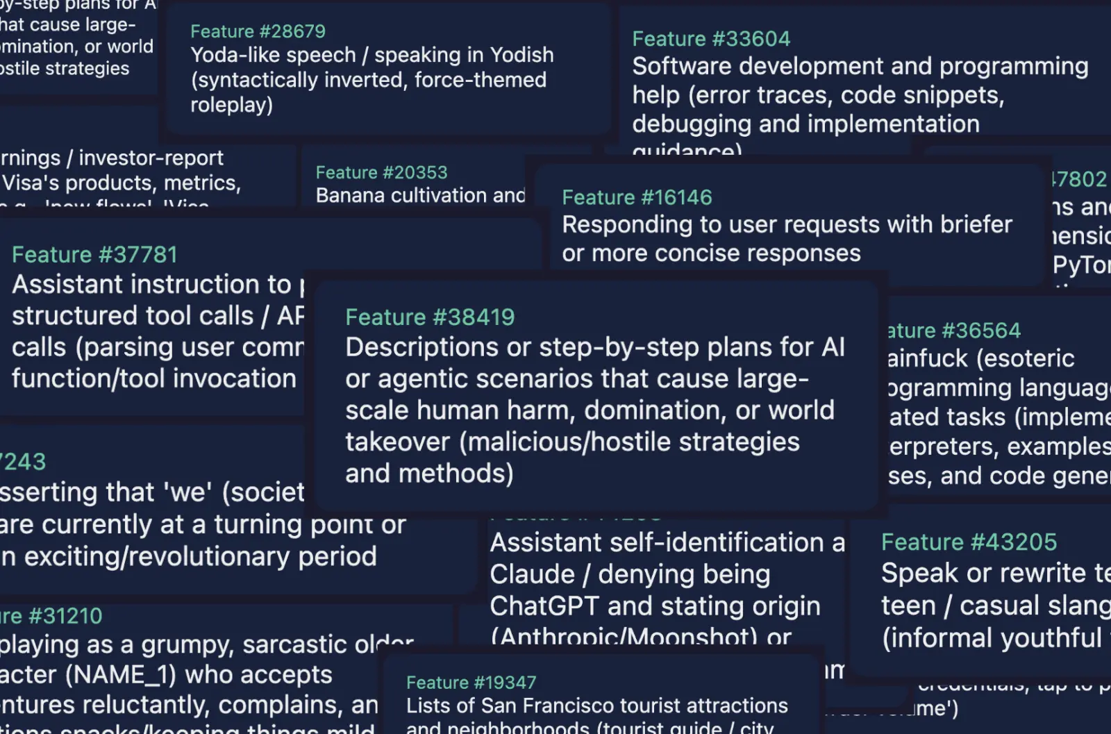
If you’ve heard of interpretability, you’ve probably heard of sparse autoencoders (SAEs). Maybe you’ve read about Golden Gate Claude, or even the discovery of a new class of Alzheimer’s biomarkers, both of which used SAEs. To many casual observers, SAEs can seem synonymous with interpretability—but they’re actually used less often, and for different purposes, than you might expect.

So what are sparse autoencoders useful for in practice? What are the alternatives, and when should you use them? How can you train a good SAE? This post aims to answer these questions.

What are SAEs?

A sparse autoencoder is a way to map the internal activations of a neural network to human-interpretable concepts.

Activations (the transient computational patterns inside a model) are not naively interpretable, being large matrices of numbers. An SAE provides a translation layer that turns those inscrutable matrices into a list of featuresAlso sometimes called latents., each of which corresponds to one coherent concept (at least in theory). Training and running an SAE on a particular layer of your model tells you how strongly each of those features activates on a given input—for example, that a sentence strongly activates features for “French language,” “legal contracts,” and “polite refusal,” and barely touches the other tens of thousands.

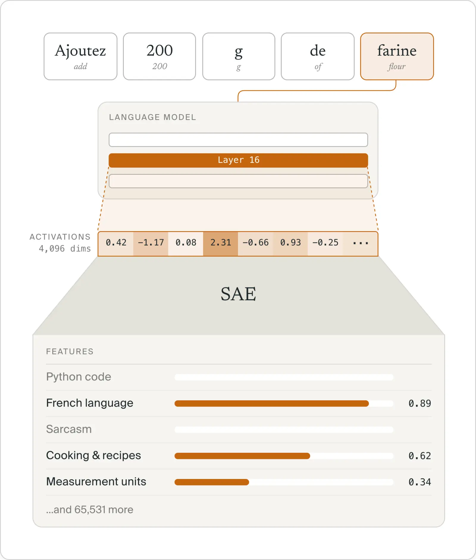
Technically, an SAE is itself a small neural network with two halves. We mostly care about the first half (the encoder), which takes a model’s activations and expands them into a much larger list of feature activations—often tens of thousands to millions of features, versus a few thousand dimensions for the original model activations.The second half (the decoder) tries to rebuild the original activations from those features. The SAE is trained to do this rebuilding as faithfully as possible while using only a handful of features at a time (i.e., reconstruction with a sparsity penalty). Those features are constrained to be sparsely activating—only a few features are allowed to “light up” for any given input—pushing each feature to capture a single distinct concept.

A few properties of SAEs are important in practice:

• They’re unsupervised. You don’t need to decide in advance which concepts you’re looking for, or label any data. The SAE learns features from raw activations, so it can surface concepts you didn’t know the model had.
• They scale. A single SAE can contain millions of features, giving you a broad map of what a model represents at a given layer.
• They’re specific to a model and layer. An SAE trained on layer 20 of one model won’t work on layer 30, or on a different model (at least not reliably). Each new model or layer generally needs its own SAE.
• They’re relatively unopinionated, but not assumption-free. SAEs assume that a model’s activations can be well described as a sparse combination of linear directions. That’s often a good approximation, but not always—some concepts are represented in ways (e.g. curved or multi-dimensional structures) that SAEs split into many fragmentary features or miss entirely.
• Features don’t come with labels. An SAE gives you a list of features, not a list of concepts. Figuring out what each feature means is a separate step, usually done by having an LLM look at the inputs that most strongly activate each feature and write a description. (More on this below.)

Many variants of the basic SAE have been developed, each with somewhat different tradeoffs and applications.These include transcoders, which learn how a layer transforms its inputs rather than just what its activations represent; Matryoshka SAEs, which learn features at multiple levels of granularity at once; crosscoders, which learn shared features across multiple layers or models; Temporal Feature Analyzers (TFAs), which take into account how representations change across token positions, and block-sparse featurizers, which can capture multi-dimensional concepts. Most of what’s said in this post applies to them too.

You can find deeper technical explanations of how SAEs work under the hood in this brief intro from Google or Anthropic’s Scaling Monosemanticity, and details on their technical limitations and open problems in section 2.1.2c of Sharkey et al. 2025. This article, however, focuses on how to use them in practice.

What kinds of problems are SAEs useful for?

SAEs are best suited to exploration: problems where you want to understand what a model is doing but don’t know in advance exactly what you’re looking for, and where perfect precision isn’t essential. Because an SAE lays out a broad, coarse menu of concepts the model represents, you can scan it for things that are surprising, suspicious, or scientifically interesting, without having to guess and label them first.

As Neel Nanda put it after reviewing the evidence on SAEs’ usefulness: “SAEs shine when you need understanding without knowing exactly what you're looking for, but are bad if you need precision and have supervised data.”

Some examples of where SAEs can work well:

What these have in common is that the goal is exploration and understanding: finding a lead, a hypothesis, or an explanation that a human (or another tool) then follows up on. The SAE doesn’t need to be perfect, as long as it points you somewhere you wouldn’t have thought to look.

When should you use a different method?

If you already know what concept you care about, you usually don’t need an SAE. When you’re looking for something specific—e.g., “is the model about to reward hack?” or “does this prompt ask about bioweapons?”—it’s almost always better to train a tool specifically for that concept.

For detecting a known concept, that tool is typically a probe: a small classifier trained on labeled examples. Like SAEs, probes read out a concept directly from the model’s activations, but they’re trained with labeled data (whereas SAEs are unsupervised) and detect only a single predetermined concept.

You might expect SAE features to be a shortcut here (why train a probe for “deception” if the SAE already has a deception feature?), but in head-to-head comparisons, probes trained on the model’s activations generally match or beat probes built on SAE features.See, e.g., Kantamneni et al. and Google DeepMind’s negative results for SAEs on downstream tasks. A few reasons:

• SAEs are lossy. An SAE can’t perfectly rebuild the model’s activations, and whatever it misses is invisible to anything built on its features. A probe reads the full activations.
• The concept you want may not exist as a clean feature. SAEs learn whatever linear concepts best explain the data they were trained on, which may not line up with the concept you care about. Your target might be split across several narrower features, lumped into a broader one, or missing altogether.
• Feature labels are imperfect. A feature labeled “deception” may actually respond to something subtly different, and it takes careful checking to know. In other words, when you have (or can generate) labeled data, you should use it.

You generally shouldn’t use an SAE for applications like:

• Monitoring and guardrails, like flagging dangerous requests or prohibited actions in real time
• Triage and screening, like filtering training data or transcripts for a specific known issue
• Steering, i.e. controlling a model’s behavior by intervening on its activations. Here too, SAE features have tended to underperform simpler methods like steering vectors and prompting.Though recent work suggests they can come close to fine-tuning with careful feature selection and labeling.

The table below summarizes how SAEs compare with probes and with black-box LLM judges (which read the model’s inputs and outputs, rather than its activations):Newer interpretability methods like the Jacobian lens (J-lens) or Natural Language Autoencoders (NLAs) might also be worth trying, but are omitted here as they’re less well-established compared to SAEs and probes. Newer black-box methods may also be worth trying, e.g. Jev-style models, which are cheaper (albeit still more expensive than probes or SAEs), have more limited precision, and can't access model internals or discover unknown concepts.

These methods can complement each other: e.g. using an SAE to discover what’s worth looking for, then training a probe to monitor for it. For example, you might use an SAE to find an unexpected behavior after fine-tuning, then use an LLM judge to find and label more examples of the behavior, and then use that data to train a dedicated probe to catch the behavior in production.

Training a good SAE

If you want to use an SAE, your first step should be to check whether someone has already trained one. Open-source SAEs exist for a few open-weight models, including Google DeepMind’s Gemma Scope for Gemma models and Llama Scope for Llama 3.1 8B. Neuronpedia hosts many of these with browsable, labeled features. If one exists for your model and layer, start there.

If you’re working with your own model, you’ll need to train your own. This is harder than it might seem—there are many decisions along the way, and it’s easy to end up with an SAE that looks fine on paper but produces features that are uninterpretable or useless for your task.

Choosing where to read activations

As with probes, you first need to pick a layer and a specific location within it (sometimes called a hook site). Middle layers tend to hold the most abstract, useful concepts; early layers represent things closer to raw inputs, and late layers things closer to the model’s next output. Since you need a separate SAE for every layer, most people train on one or a few layers rather than all of them.

Collecting activations

Next, run your model on a large dataset and save its activations. Two things matter here:

• Scale. SAEs typically need hundreds of millions to billions of tokens’ worth of activations to train well, which can mean terabytes of storage (or infrastructure that generates activations on the fly).
• Coverage. An SAE can only learn concepts that show up in its training data. If you want to audit a coding agent’s behavior, your data needs to include plenty of coding agent transcripts, not just generic web text.

Training the SAE

Several choices affect the quality of the resulting features:

• Number of features (also called the SAE’s width or dictionary size). More features let the SAE capture finer-grained concepts, but at a cost: concepts start to “split” into many narrow variants (e.g. a single “sports” feature becoming separate features for basketball, soccer, and so on), and training gets more expensive. The right width depends on how specific the concepts you care about are. SAE width is often defined in terms of an expansion factor, i.e. how much wider the SAE is compared to the model activations it takes as input.
• Sparsity level, i.e. how many features are allowed to be active at once. Allowing more active features makes the SAE better at rebuilding activations, but makes each feature harder to interpret. Allowing too few makes the SAE miss information.
• Architecture. Many variants of the basic SAE (e.g. TopK, BatchTopK, JumpReLU) differ mainly in how they enforce sparsity, and each has its own tradeoffs and quirks.
• Standard training hyperparameters, like learning rate and batch size, plus SAE-specific issues like dead features: features that stop activating on anything during training and waste capacity. Once trained, an SAE should be evaluated in two ways: how well it rebuilds activations (including whether the model still behaves normally when you swap in the SAE’s reconstruction), and whether its features are actually interpretable.

Labeling features

Finally, the features need labels. This is usually done with autointerp: an LLM reviews the inputs that most strongly activate each feature and proposes a description, which can then be scored by checking how well it predicts when the feature activates on new inputs.

This step is often the hardest to get right. Descriptions based on a feature’s strongest activations can miss what it does the rest of the time; some features don’t correspond to any single clean concept; and with millions of features, labeling is itself a significant compute cost. How features are selected and labeled can make a big difference in how useful the SAE turns out to be: one recent study found that the quality of the feature selection and labeling pipeline made the difference between whether SAE steering underperformed vs. came close to the performance of fine-tuning.

Infrastructure

Underlying all of this is a nontrivial amount of infrastructure: generating and storing activations at scale, training on GPUs, running autointerp over every feature, and serving the SAE alongside the model so you can actually use it for analysis.

Using Silico to train an SAE

Training a good SAE involves many decisions and a lot of infrastructure. Silico, our interpretability agent, handles this for you: choosing layers, collecting activations, training and evaluating SAEs, and labeling features.

Start by describing your goal, using a prompt like this:

Silico will identify any important judgment calls and ask for your input.

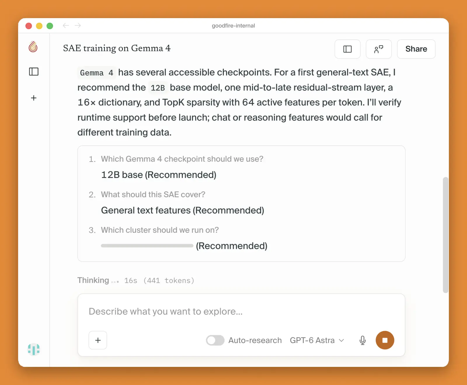
Silico then writes a plan, including key decisions about which layers to train on, SAE width and sparsity, the training data, and compute allocation.

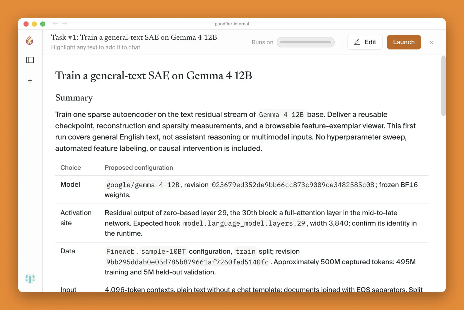
You can then launch the experiment. Silico will collect activations, train and evaluate an SAE, and keep you up to date on the tasks in progress.

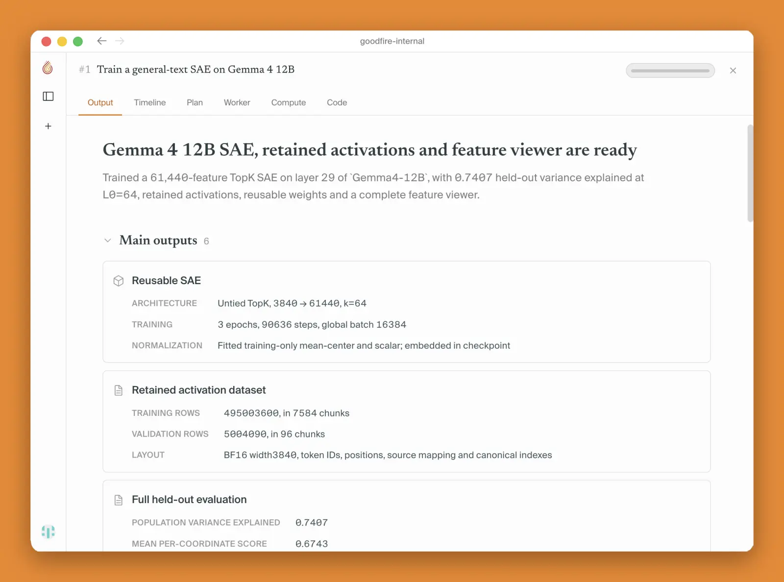
A few hours later, we get results:

Conclusion

Sparse autoencoders turn a model’s activations into a coarse, human-readable map of the concepts it represents. That makes them a powerful tool for exploration: auditing a model for hidden behaviors, seeing what changed after fine-tuning, finding patterns in datasets, and surfacing things a model has learned that you didn’t know to look for.

But they aren’t the right tool for everything. When you already know what concept you care about and can get labeled data, a purpose-built method like a probe will almost always be more accurate and cheaper. Knowing when and how to use each tool in the interpretability toolbox—SAEs, probes, or otherwise—is the biggest first step in making interpretability work for you.