Abstract
A companion to Neural Networks Are Already Clean
An intuitive way to interpret a neural network is to study its neurons; that is, the hidden units of its MLP layers. However, they have long appeared too complex and polysemantic for direct study. This view has led much of the field to focus on learned feature spaces over sets of neurons, which makes interpretability more challenging: we first need to transform the model before normal science can begin.
Building on a growing body of literature, our work suggests that neurons are more interpretable than previously assumed. We study the neurons of Qwen3.6-35B-A3B using sparsification methods, attribution tools, and research agents, and find three properties that make neurons interpretable units of computation:
First, they are already functionally sparse. Ablating the 92.2% weakest MoE neuron activations for each forward pass has only modest effects on model capabilities – a 2.9% increase in language model loss.
Second, neurons have relatively few semantic groupings (modes) of computational functions, and we can identify these and describe them concisely. The majority of neurons have either one mode only or a single mode that is overwhelmingly causally significant. In cases where multiple causal modes are present, the number is small and legible to our methods.
Finally, we can use agent-driven experimentation to generate neuron descriptions in natural language, and these descriptions allow us to predict, simulate, and activate the neuron. Providing the description to a judge model allows us to (1) predict whether the neuron will fire in a given passage of text with 95% accuracy vs random text; (2) simulate its token-by-token behavior in high-activation regimes sufficiently to recover 73% of the damage (as a proportion of a ceiling of damage restorable) from the neuron’s ablation; and (3) write text that causes the neurons to fire more strongly than anything observed in a 10B-token corpus.
Overall, we argue that neurons are meaningful units of computation that can be effectively used for interpretability in their own right, letting us study the model on its own terms rather than through a learned proxy.
Introduction
In the previous essay in this series, we argued that neurons in deep learning models are more interpretable and cleaner than has often been suggested. In this article, we describe what this means in more detail and share our empirical findings. Throughout, the term “neuron” refers to an individual computational unit in the intermediate layer of a transformer MLP, whose output is a scalar activation, computed after the nonlinearity (SiLU), as explained in the Background section below.
Neurons were the first units through which deep networks were interpreted, and early work found them to be closely aligned with recognizable concepts (Le et al., 2012; Zeiler & Fergus, 2014; Bau et al., 2017; Olah et al., 2017; Radford et al., 2017; Goh et al., 2021). However, this story was complicated by observations of so-called polysemanticity—the idea that individual neurons respond to seemingly unrelated inputs (Nguyen et al., 2016; Olah et al., 2020). Polysemanticity is related to the proposal that more concepts are represented in a network than the number of neurons in the network, an idea canonized in the literature on “superposition” (Elhage et al., 2022; Arora et al., 2018; Park et al., 2023; Costa et al., 2025). This, in turn, led to the development of learned overcomplete feature dictionaries in place of neurons as computational units of analysis (Bricken et al., 2023; Cunningham et al., 2023). Despite these trends in the field, interpretability researchers continued to investigate respects in which neurons may still constitute a meaningful unit of analysis (Geva et al., 2021; Dai et al., 2022; Geva et al., 2022; Gurnee et al., 2024; Arora et al., 2026; Dravid et al., 2026; Feucht et al., 2026; Shabalin & Piotrowski, 2026). We continue this line of work, introducing new ways to factor and understand what individual neurons compute.
Whether a neuron is labeled monosemantic or polysemantic can depend on choices about what constitutes a single concept, and responses that initially appear unrelated may share a regularity that becomes apparent with a better understanding of the computations they support (Murphy & Medin, 1985). We therefore characterize neurons by their computational functions as our primary object of study, considering semantic similarity of the texts that activate them as a secondary question. We study the circuits in which each neuron participates, tracing how upstream neurons drive its activation and how downstream neurons use its output. This lets us examine how a neuron’s role varies across contexts and assess whether those roles admit a concise description.
A common view is that neurons are an intractable unit of analysis. In the worst case, an investigation could have demonstrated this in three ways: (1) Individual neurons might rarely play identifiable computational roles, so that meaningful units would be clusters of neurons, or directions and manifolds in activation space; (2) Each neuron might take extreme values on a wide and heterogeneous range of inputs that no short description unifies; (3) Or neurons might resist descriptions precise enough to predict when, and how strongly, they fire. We test each possibility directly: we ablate weak activations, determine the semantic range of neurons’ computational roles, and predict and simulate activations from descriptions alone.
Our results provide evidence that neurons are tractable units of analysis. Neurons (1) exert most of their downstream influence in high-activation regimes (above the 97th percentile at the positive extreme and below the 3rd at the negative); (2) have a small number of computational roles, distinguished by their interactions with other components of the network; and (3) can be given concise descriptions that predict and simulate their activations. The three results share a pattern: the stronger a firing, the more the model depends on it and the more precisely we can describe it.
The picture that emerges is not that every neuron means one thing, but that a neuron’s important firings have a small set of computational functions, and a short description captures them. Some neurons are genuinely polysemantic, and some behavior remains unexplained, but so far little of it appears critical for the model’s computation.
We therefore find that neurons are a useful and interpretable basis for understanding LLMs.Some Definitions
One neuron, one token
- Write
- The neuron's contribution to the residual stream, a · wrouter · Wdown[:, n]: its column of the down-projection matrix, Wdown[:, n], scaled by its expert’s router weight, wrouter, and the output of its SwiGLU activation function, a.
- Activation
- The combined scalar a · wrouter.
- Pole
- As we explain below in more detail, modern neurons’ activation functions can produce a positive or negative value. A pole is the positive or negative extreme of a neuron, and usually (but not always) positive and negative values have unrelated roles.
- Firing
- A fire is an individual event in which a neuron's activation on a particular token is nonzero (on the positive or negative pole). In an MoE model this requires that the token was routed to the expert containing the neuron. These neurons do not have true “off” values since they are never 0, and in practice most activations are very weak (hence our focus on strong activations).
- p97/3, p99/1, etc.
- We use this notation as shorthand to refer to the percentile of a neuron’s activation relative to all its activations across a corpus. On this scale, p1, p5, etc. are negative activations (as the median activation of neurons in this study is near 0). Thus, p97/3 refers to both positive and negative extremes, p3 ∪ p97.
How neurons connect
- Input neurons
- Every neuron receives input from a large set of “causally upstream” neurons, which we refer to as inputs. In particular, to serve as input, a neuron from a previous layer must either 1) produce an output vector, written to the residual stream, that is aligned with the target neuron’s gate or up weight matrix; or 2) be identifiable through attribution techniques as having an effect on our target neuron, mediated by attention.
- Reader neurons
- The inverse of input neurons. A reader neuron is a neuron that responds to whichever neuron we are discussing, either directly or through attention.
- Circuit
- A computational subgraph of the entire network that is causally sufficient for producing a given output. In this article, we focus on circuits that use individual neurons as nodes.
- Subcircuit
- A computational function that consists of a set of input neurons and reader neurons where the two sets are connected through a single target neuron. A neuron can host multiple subcircuits and they can exist simultaneously. However, because the members of a subcircuit are highly disjoint from the members of other subcircuits, only one is active at a time.
What a neuron means
- Response profile
- The pattern of textual features and concepts a neuron fires on across a dataset.
- Max-activating examples
- Texts that cause a neuron to fire near the top of its activation range; i.e., to output a value that is one of the strongest observed for the neuron.
- Computational function
- Neurons can receive input from potentially thousands of other upstream neurons, and are read by potentially thousands of downstream neurons. A computational function is a description of the causal process by which a set of identifiable inputs is transformed into a meaningful output; a simple example would be “combines location and cultural cues from upstream neurons to output a signal that Tokyo is being mentioned.”
- Mode
- A semantic grouping of computational functions (subcircuits) of a neuron. Neurons with more than one mode are referred to as multimodal.
- Mono- and Polysemanticity
- These terms conventionally describe a neuron that responds to a single “concept” or to multiple seemingly unrelated “concepts”, respectively. However, as discussed in the section below (see “Moving from Polysemanticity to Computational Role”), these labels admit multiple interpretations, and the apparent semantic coherence of a neuron’s responses does not by itself determine its computational function. We therefore focus on how downstream neurons use its signal.
This is the first in a series of technical articles exploring neuron interpretability. This post introduces our initial findings and sets the frame for further exploration.
Our primary findings are as follows:
- Language models can operate under considerable neuron sparsity. Inspired by the foundational work of Arora, Wu et al. (2025), we evaluate several sparsification methods according to (1) KL divergence from the intact model over large datasets of natural text and (2) benchmark performance.
- By ablating all neuron firings below extreme activations (correcting for the bipolarity of gated neurons, as explained below), we show that the aggregate causal role of a model's neurons can be attributed largely to the activations in the highest ranges–specifically, the 97th percentile and above and the 3rd percentile and below for negative values, p97/3 in our notation. This range is precisely where neurons are most interpretable. Up to 92.2% of the weakest absolute neuron activations can be ablated either through top-K or percentile-based filtering with only small effects on loss, KL, and a broad set of performance benchmarks. Further, those negative effects on benchmark performance can be corrected with only 91M tokens of SFT and 9M tokens of RL to re-calibrate reasoning.
- Individual neuron poles have a small set of distinct computational functions that usually fall into one or a handful of semantic categories, like “beetle and insect-wing anatomy terms” or “Chinese health and wellness vocabulary.” We identify these functions by examining the upstream neurons that drive a firing and the downstream neurons that use its signal, and call a neuron’s coherent groups of functions “modes.” Coherence is defined by LLM judges classifying functions into specific categories and performing held-out example matching.
- We identify disjoint subcircuits that a neuron participates in and cluster those subcircuits into distinct modes, and find that there is more circuit similarity within modes than between modes.
- For the majority of neurons, we find either only one mode or a single dominant mode responsible for >=90% of its causal effect across a broad dataset.
- Modes have degrees of relatedness, and are not always completely unrelated semantically. For example, a neuron may have multiple Python-related coding modes, or it may have a mathematical mode and one related to Japanese honorifics. Usually, even when there are multiple modes, one is far more causally relevant than the others.
- The computational roles of neurons can be concisely described in natural language and these descriptions can be used to predict, disambiguate, and simulate neurons across a range of tests. We evaluate neuron descriptions through detection (will a neuron fire in a short token span?), classification (when a neuron with multiple semantic modes fires, can we tell which meaning is operative?), input synthesis (can we create a text that makes the neuron fire strongly?), and simulation (can we replace the neuron’s natural activations in a sequence with those based on a description of the neuron?).
- In the activation percentiles that our sparsity experiments suggest are most important for the model's primary computations, we can achieve considerable understanding of the neurons’ behavior. As activation strength rises, we are able to make more precise predictions and simulate their effects more accurately.
- For percentiles stronger than p97/3, we can detect when a neuron will fire on a short sequence 95% of the time when comparing the activating text to a random text, and 89% when comparing to a text assigned to the same expert (chance in both cases is 50%). We can also tell a neuron's modes apart, either from the circuit, by observing which downstream neurons a firing moves (its readers; one-vs-rest AUROC 0.99), or from the text alone, by giving a language model the mode descriptions (AUROC 0.95).
- For percentiles above p99.9, we can simulate neuron behavior well enough to recover 73% of the recovery achievable by a perfect reader. We note that this was achieved without any training of a model to accomplish this task. Bands p99.9 through the top activations are responsible for 73% of all neuron damage when a neuron is ablated, and thus hold the most causal significance. We ablate these neurons from all tokens in a held-out sequence and measure the KL divergence of the logits. We then replace the activations with simulated values provided by a judge LLM based on the neuron’s description. On average, this is sufficient to recover 73% of the KL damage that the perfect-reader ceiling restores.
- For 94% of neurons, we are able to generate texts that activate the neuron beyond the maximum level found in a 10B corpus of mixed pretraining and post-training data. Our descriptions capture what activates the neuron effectively, though this is only a test of each neuron’s primary mode.
Neuron Sparsity and Effective Range
The two central questions of this section are:
- Are individual neurons, instead of distributed directions spread across many neurons, the right basis for analysis of MLP computation? High levels of sparsity in MLP computations would suggest that neurons carry significant parts of the computation on an individual basis.
- What sorts of neuron activations are meaningful and necessary for computation – do strong activations suffice, or are weak activations indispensable? A highly sparse regime would suggest much higher importance for strong activations.
If the conceptual primitives for transformer computation tend to be spread out among vast arrays of neurons in a distributed code, we should expect high levels of sparsity to sabotage these computations. On the other hand, if neurons tend to be privileged, meaningful units of computation, we should expect these primitives to be more localizable and sparse.
Earlier work has observed that neurons are often quite interpretable and consistent (across activation examples) in their strongest activations, but much more diverse and hard to understand at weaker levels (Szegedy et al., 2014; Morcos et al., 2018; Zhou et al., 2018; Leavitt & Morcos, 2020; Ghorbani & Zou, 2020; Dhamdhere et al., 2018). This motivates the concern: what if weak activations are both indispensable and uninterpretable?
We find that models can still perform surprisingly well even when all weak activations (e.g., between the negative and positive extremes of p10 and p90, or even p3 and p97) are mean-ablated, achieving close to parity with the intact model on a number of non-reasoning benchmarks. More importantly, we test an ablation where every layer retains only the top-320 neurons (out of 4,096 routed neurons) by absolute activation strength for a given step of inference, ablating 92.2% of routed neurons, and show that this model performs comparably to the base model on non-reasoning benchmarks.
For all experiments, we leave the shared expert neurons unchanged, since these neurons are effectively always on and function differently from the expert neurons. In total, the shared experts make up 20,480 of the model’s 5.26 million neurons (~0.4%).
For reasoning benchmarks, we observed that the ablated model would often run into reasoning loops and self-check excessively, never completing its answer–though by checking its reasoning output, we were able to determine that the correct answers were present. With a brief fine-tuning step, we corrected the reasoning errors and met or exceeded the original model’s performance on a broad set of thinking-based benchmarks for question-answering, code, reasoning, and math. Considering that the fine-tuning tokens used were a small fraction of a typical post-training run, this provides evidence that the fine-tuning primarily corrected reasoning rather than adding new information to the model, and that the majority of the information required for performance on benchmarks was present at the higher activations.
We provide further evidence for sparsity in the Appendix: we preserve specific model predictions with even fewer neurons using the gradient-based attribution method, RelP, and we elaborate on recent findings (Shabalin & Piotrowski, 2026) showing that transcoder replacement models tend to discover neuron-localized features even when not constrained to do so.
Sparsification by Activation Strength
Our first set of neuron sparsity experiments uses neuron activation strengths to determine which neurons to ablate. We consider three methods—mean-ablating (on an individual neuron basis, across all neurons in the model) the central percentile bands of neuron activations, expert top-k filtering, and layer top-K filtering—and measure their effects on loss, KL, and a range of benchmarks. The ablated bands are symmetric in percentile rank around the median: i.e., p1 is a strong negative activation, p99 is a strong positive activation, and weak bands are p10-p90, p25-p75, etc.
Ablation Within Top Percentiles
A natural experiment is to start with the weakest neuron activations and ablate them during inference, measuring the resulting loss and KL divergence. Since SwiGLU neurons are bipolar and neurons have different activation strength distributions, we compute neuron activation strength percentile bins and apply mean ablation to everything between the positive and negative extremes (Li et al., 2023a; Liu et al., 2023a; Mirzadeh et al., 2023; Zhang et al., 2022; Liu et al., 2024; Lee et al., 2024; Jaszczur et al., 2021; Ahmad & Scheinkman, 2019; Makhzani & Frey, 2013; Song et al., 2024; Zhang et al., 2024; Wang et al., 2024; Song et al., 2023; Alizadeh et al., 2023; Zhang et al., 2023). These initial experiments were conducted without the router weight scaling, and the percentiles shown likewise do not include this scaling.
Top-K Filtering
Inspired by Shabalin & Piotrowski (2026), we attempted to find a more sparse regime by applying a top-K function (based on raw neuron activations) across each of the experts in the model. We tested top-32 and top-64, which retain 6% and 12% of routed neurons per token respectively. Experts have 512 neurons each. In practice, the top-64 neurons primarily lay at or beyond the p5 and p95 extremes (Sun et al., 2024; Dettmers et al., 2022; Kovaleva et al., 2021; Puccetti et al., 2022; Bondarenko et al., 2023; Olshausen & Field, 2004). As with the ablation within top percentiles, this was performed without the router weight scaling.
Router-Weighted Top-K Filtering
To account for expert router weighting, we apply our activation definition above and score each routed neuron by its router-weighted activation. We then apply a single top-K over all 8 × 512 = 4,096 routed neurons of each token rather than one per expert, so the budget can shift toward experts whose neurons have the strongest activations after router weighting. We keep the top 320 (7.8%) of routed neurons (40 per expert on average, 92.2% sparsity) and zero the rest before the down projection. Here, most activations exceed the p3 and p97 extremes. Like other activation-sparsity methods, the mask is computed from each token’s own activations at inference time and needs no training (Liu et al., 2023; Lee et al., 2024; Liu et al., 2024; Wang et al., 2024; Makhzani & Frey, 2013).
Performance Under Ablation
We found that the model was able to operate surprisingly well under high levels of sparsification. Below, we show the sparsified models’ loss and KL divergence, as well as performance on a wide range of benchmarks:
| Metric / benchmark | Base model | Sparsified models | Baselines (controls) | ||||||
|---|---|---|---|---|---|---|---|---|---|
| Expert top-K | Layer top-K | Band ablated | Random | Inverse of Top-64 | |||||
| Top-64 | Top-32 | Top-320 | P25–P75 | P10–P90 | P5–P95 | Random-64 | Bottom-448 | ||
| Web text (8.4M tokens) | |||||||||
| Cells ablated | 0% | 87.5% | 93.8% | 92.2% | 49.7% | 78.6% | 88.8% | 87.5% | 12.5% |
| Loss | 1.886 | 1.952 | 2.032 | 1.940 | 1.896 | 1.926 | 1.977 | 4.214 | 4.587 |
| Δ loss | 0 | +0.066 | +0.146 | +0.054 | +0.010 | +0.040 | +0.091 | +2.328 | +2.701 |
| KL | 0 | 0.152 | 0.263 | 0.140 | 0.033 | 0.088 | 0.162 | 2.511 | 2.885 |
| Classic suite · Δ accuracy vs base model, percentage points (acc; GSM8K strict match) | |||||||||
| ARC-Challenge | 54.9 | +2.0 | +1.5 | +0.3 | −0.7 | +1.3 | +1.8 | −32.8 | −37.3 |
| ARC-Easy | 81.4 | +0.8 | +1.5 | +0.2 | +0.6 | +1.7 | +2.1 | −40.3 | −49.1 |
| WinoGrande | 73.9 | −1.4 | −2.0 | −2.2 | +0.1 | +0.2 | +0.3 | −23.2 | −23.6 |
| HellaSwag | 57.4 | −0.7 | −1.1 | −1.6 | −1.1 | −1.3 | −1.7 | −25.5 | −26.9 |
| MMLU | 84.2 | −1.6 | −3.4 | −1.2 | −0.4 | −0.7 | −1.8 | −60.1 | −60.9 |
| GSM8K | 96.7 | +0.3 | −16.7 | −1.7 | −1.0 | −1.3 | −9.3 | −96.3 | −94.0 |
| Thinking evals · Δ accuracy vs base model, percentage points | |||||||||
| SuperGPQA | 44.8 | −15.2 | −17.9 | −13.0 | +0.9 | −8.1 | −14.4 | −44.5 | −44.6 |
| MMLU-Redux | 91.5 | −3.7 | −5.8 | −3.0 | +1.0 | −2.7 | −5.0 | −89.0 | −90.4 |
| MMLU-Pro | 78.4 | −8.5 | −18.9 | −8.3 | +0.2 | −4.3 | −13.0 | −78.0 | −78.0 |
| IFEval | 30.9 | −0.6 | −0.4 | +0.4 | +0.0 | +0.0 | +0.4 | −15.9 | −15.2 |
| MedQA | 92.8 | −7.8 | −16.0 | −4.6 | +0.8 | −2.5 | −4.1 | −83.9 | −80.6 |
| GPQA-Diamond | 63.6 | −18.2 | −25.8 | −11.1 | +2.5 | −10.6 | −20.7 | −54.0 | −55.6 |
| MATH-500 | 69.8 | +7.0 | −4.0 | +5.8 | −3.8 | −3.2 | −12.8 | −69.8 | −69.8 |
| AIME 24+25 | 0.0 | +11.7 | +3.3 | +11.7 | +1.7 | +3.3 | +1.7 | +0.0 | +0.0 |
| HumanEval+ | 59.1 | +7.9 | +3.0 | +15.9 | −7.3 | −20.7 | −33.5 | −59.1 | −59.1 |
| MBPP+ | 71.7 | −20.4 | −24.9 | −20.9 | +5.6 | −12.2 | −14.8 | −71.7 | −71.7 |
Table 1: KL, loss, and benchmark performance under sparsification. Base model benchmark scores are percentages; other benchmark columns show changes in percentage points. Red indicates a decrease; blue indicates an increase. Zero is white. There is a far smaller drop in performance from retaining the top-K neuron activations, either per layer or per expert, as opposed to the complement or random-64; the latter two destroy performance. Ablation based on percentile bands similarly retains a disproportionate amount of performance on the top bands. Note that the P25–P75, P10–P90, etc. percentile bands were computed without router-weighting, unlike the percentile bands referred to throughout the remainder of this text.
Performance is retained to a surprising degree across benchmarks, especially when compared to controls. The ablated models retained high performance across classic benchmarks like ARC-Challenge, ARC-Easy, WinoGrande, and HellaSwag, improving slightly on some evals and dropping on others. However, we observe drops in reasoning and knowledge-based evals. When we observe rollouts directly, we see that the sparsified model’s reasoning tends to loop and self-check excessively. However, when we classified these rollouts with Claude Opus 5.5 agents, we identified that the sparsified model would still mention the facts and correct answers, usually as the last answer candidate–it would just self-check endlessly afterwards. We further found that reasoning collapse seems related to the double-negative activations we discuss in the next section, since restoring those specific activations restored reasoning.
In order to see if this strong-activation regime could recover full benchmark performance, we follow Shabalin & Piotrowski and perform light fine-tuning on the layer top-320 model and re-measure performance; across benchmarks we were able to see full restoration of function. We discuss methods and results further in the Appendix section Extended Sparsity Results and Discussion.
What we suggest, then: the original model is very close to sparse, with most of the computation located in the top activations. This implies that even the original model is likely quite interpretable and causal at the top ranges, but also that it is relatively easy to tip a model over the edge to more complete sparsity. Our subsequent analyses of neurons in the fine-tuned model showed that the neurons retained their original functions, remained interpretable, and had the same numbers of modes.
Principled Selection of a High-Activation Band
Most of the model’s functionality is retained after top-320 layerwise filtering, and that lost performance is easily restored with light fine-tuning. The retained router-weighted activations fall almost entirely in the p97/3 band. We therefore use this activation regime for the experiments covered in the remaining sections.
Sparsity takeaways and the interpretable regime
We now have evidence from several directions suggesting the following:
- The set of neurons required for each step of inference is surprisingly sparse. General sparsification methods like top-K achieve comparable benchmark performance at ~92.2% sparsity; as we discuss in the appendix, specific circuit-finding tools produce even greater sparsity.
- Retained neurons are almost always firing at the positive and negative tails, often p97/3 or stronger.
- Double-negative/Q3 activations seem to consist of a functionally different regime. Though we did not analyze it in detail, we expect that it is likely that it is approachable with further investigation.
From this evidence, we conclude that even if we do not fully understand weak activations, we can nevertheless understand the bulk of what the MLPs are doing if we limit ourselves to examining the tails. Weak activations may not be entirely irrelevant, and may perform a function, but we leave investigation of them to future work.
We further hypothesize that the sheer sparsity of neuron activations in these experiments suggests that neurons constitute a privileged basis, that they are meaningful units of analysis, and that the connections between them can help elucidate their functions.
Now that we have laid the groundwork for investigation of the neurons’ positive and negative extremes, the next question is: what does their behavior in these regimes tell us?
Understanding Neuron Computations
Moving from Polysemanticity to Computational Role
Neurons are often thought to be difficult to interpret because a single neuron can respond to several seemingly unrelated concepts. This property, known as polysemanticity, has been described in terms of responses to unrelated latent variables, mixtures of inputs, or multiple semantic concepts (Olah et al., 2020; Bricken et al., 2023; Bills et al., 2023).
These informal definitions do not resolve what makes concepts distinct. Whether a neuron is labeled monosemantic or polysemantic can depend on choices about what constitutes a single concept (Murphy, 2002). As noted in Neural Networks Are Already Clean, humans tend to describe neurons as detectors for groups of nouns. But categories do not always follow this principle. Klindt et al (2026) compared this phenomenon to the New York Times Connections Game, where the objective is for users to group words by non-obvious similarities, and Barsalou, 1983 famously illustrated this with goal-derived categories such as “things to sell at a garage sale”. An old GameCube and an unused kayak seem to have little resemblance, but they would both belong to this category. Recognizing a unifying concept also depends on the interpreter’s background knowledge (Murphy & Medin, 1985). Responses that initially appear unrelated may share a regularity that becomes apparent only with a better understanding of the computations they support.
An alternative approach is to investigate neurons from a computational perspective first, rather than beginning with semantics. How do different sets of input neurons make a neuron fire, and how do downstream reader neurons use a neuron’s signal? By identifying distinct computational functions that a neuron performs, we can develop objective, quantitative tools to analyze a neuron; and we can then examine their semantics to map computational functions back to interpretable concepts. This approach makes it possible to demystify neurons even when they perform multiple or confusing computations, because the subcircuits involved remain legible. And as long as these roles are few and concisely describable, we can still understand the neuron by characterizing each role and the contexts in which it operates (Rigotti et al., 2013; Fusi et al., 2016; Quiroga et al., 2005; Barlow, 1972; Marr, 1982). This allows us to retain the neuron as a unit of analysis even when it serves multiple distinct computational roles.
We therefore adopt this approach–first looking at computational function, and only then examining semantics–as our primary investigative procedure. In our next section, we describe precisely how we perform this analysis.
Understanding Neuron Computation via Subcircuits
We intentionally target the high-activation regimes that our sparsity experiments demonstrate to be the most causally important (p97/3 and stronger). As motivated above, our approach here is computational/functional rather than semantic: rather than understanding a neuron in terms of the types of texts that activate it, we instead examine what function the neuron plays in network computation. In particular, a neuron is interpreted in terms of its upstream and downstream connections to other neurons.
We extract various subcircuits that a neuron participates in as the language model processes input text. We define a subcircuit as a computational subgraph with a set of input and reader neurons that connect through a target neuron, and seek to identify disjoint subcircuits that run through the neuron. A neuron participates in multiple subcircuits, each implementing a unique computation through the gate ⊙ up multiplication. A neuron always writes to the same direction in the residual stream. However, the same textual context that causes the neuron to fire can also prime different downstream neurons to read the original neuron’s signal.
An analogy can be made to the signal processing idea of multiplexing, where multiple signals from different subcircuits are compressed into a single channel (Lee & Messerschmitt, 1988; Mante et al., 2013; Rigotti et al., 2013; Salinas & Thier, 2000; Dreyer et al., 2024; Gandelsman et al., 2024). A single neuron may serve as a shared channel for different computations, with the surrounding context determining how downstream neurons use its signal. This is made particularly easy by the nature of gated MLPs, since upstream neurons can perform a switching function to activate different sets of readers depending on the context through a combination of the gate and up projections. We discuss this in the text on disambiguation below.
Subcircuit multiplexing
One routed-expert neuron in Qwen3.6-35B-A3B. Example contexts are illustrative.
Figure 5: An illustration of how neuron subcircuits work. The neuron output vector is always the same direction, but by priming different downstream reader sets, the neuron can be used for different functions.
Identifying Computational Functions From Subcircuits
To identify these subcircuits, we first ran 10 billion tokens from diverse domains through Qwen 3.6 35B-A3B including data from pretraining, reasoning, chats with users, and math. For each of the model’s 5 million neurons, we collected 1,000 examples from each of 14 activation percentile bands, for a total of 14,000 examples per neuron. We then collected an additional 30,000 examples per neuron for a stratified subset of 2,734 neurons. These additional examples were drawn from p97/3 and stronger. As a starting point for neuron descriptions, we used a fine-tuned Qwen3-8b model to produce basic labels for each neuron based on example sentences the neuron fires on.
To identify subcircuits, we first characterize each firing by its upstream inputs. With each layer’s RMSNorm scale held at its actual value, the target neuron’s gate and up pre-activations decompose exactly into direct contributions from the residual-stream writes of earlier neurons. We keep the inputs that contribute most. To collect downstream readers, we propagate the target neuron’s write along the residual stream to every later layer at the same position, through the same frozen RMSNorm. We estimate each reader neuron’s change in activation to first order. See the Methods section in the Appendix for details.
We then profile each firing by the inputs that drive or suppress its gate and up projections. For each projection, we subtract each input’s mean absolute contribution across the expert’s neurons from its absolute contribution to the target neuron, then retain the 400 top inputs for each of the gate and up projections. We separate these inputs into two bins: those that support the sign of the projection’s pre-activation and those that oppose it. This gives each firing a profile with four parts: gate drivers, gate suppressors, up drivers, and up suppressors. Keeping these separate lets us distinguish firings where the same input plays different roles–for example, an input neuron could suppress one subcircuit through the gate, or activate another subcircuit through the up projection.
We next compare these profiles across firings of the same pole to identify upstream subcircuits that recur in different contexts. Inputs that appear in nearly every firing provide little information about what distinguishes one firing from another. We therefore weight the profiles with TF-IDF to downweight common inputs, and normalize the four quadrants so that each contributes equally. Since we do not know in advance how many subcircuits a pole has, we use community detection to find groups of firings with similar input profiles. We split examples by document, using 75% of documents for fitting and holding out the remaining 25% for evaluation. We connect each firing in the fitting set to its 15 nearest neighbors by cosine similarity of the input profile, then run the Leiden algorithm, a community detection algorithm. Each held-out firing is assigned to the group whose centroid is nearest in cosine similarity.
This procedure can split a single circuit into several groups. To bring these back together, we merge groups when their top 50 input neurons overlap by at least 30% and their top 50 downstream readers also overlap by at least 30%, a heuristic that we find produces higher-quality subcircuits. Requiring agreement on both sides helps ensure that the merged groups reflect the same underlying circuit.
This yielded a median of 19 subcircuits per pole (with a range between 1 and 51), with low overlap in their inputs and readers. We send each subcircuit, with a description of its inputs and readers, to Claude Opus 5.5 to produce a concise description of the subcircuit.
We see that subcircuits are highly disjoint:
| Top-50 overlap between subcircuits of one neuron | Inputs | Readers |
|---|---|---|
| Mean over all pairs | 5.2% | 6.5% |
| Typical pair, the median | 2% | 2% |
| Nearest neighbor, the median | 14% | 17% |
Table 2: Set overlap for input and reader neurons for subcircuits within a neuron. The nearest neighbor is the subcircuit with the most overlap within a neuron.
For each subcircuit, we obtain three different descriptions. The first describes how upstream neuron inputs through the gate and up projections cause the neuron pole to fire. The second describes how the subcircuit appears in text alone. Finally, we also describe the token pattern: what actual tokens in a text does this neuron fire on?
The three parts of a subcircuit description
Corneal haze and stroma in LASIK/PRK refractive surgeryNeuron L9_E220_N343, positive pole, subcircuit c1
GateOpens on corneal tissue-condition and opacity units (vascularization/infiltration, opacities/clouding, 'haze', epithelial fragments).
UpWrites positively from tissue-pathology, dystrophy and 'haze' units.
Corneal refractive laser surgery (LASIK, PRK, excimer laser ablation of the corneal stroma), peaking on its post-op complication and anatomy terms: corneal haze, corneal stroma, ablating, excimer laser.
Fires mostly on the token right after 'corneal' or 'H'. Examples are 'haze' in 'corneal haze' / Chinese 'Haze' and 'st' in 'stroma'.
Inputs, firings and full descriptions
- L8_E227_N440eye opacity and clouding
- L7_E84_N177pieces of technical and scientific terms
- L1_E228_N340the word “haze”
- L7_E84_N43tissue vascularization and infiltration
- L7_E84_N492degenerative tissue conditions, dystrophy
- L1_E64_N125technical and mathematical expressions
- 24×节约了大量角膜厚度,显着减少了术后Haze的发生,超薄LASIK手术术后
- 22×factor (CRF), and cornealhaze. ⏎Results: This study was
- 21×a hinge, ablating the cornealstroma in a refractive correction amount
- 20×with significant side effects such as cornealhazeand regression. Several factors have been
Lines are the upstream neurons that most drive this subcircuit's gate and up projections; width is attribution. On the right are its four strongest firings, with the firing token underlined and every token shaded by activation; the number is the activation as a multiple of the firing threshold. The neuron multiplies its gate, after SiLU, by its up input. This subcircuit is 212 of the pole's 5,000 sampled firings.
Circuit
Combines corneal-tissue pathology signals (vascularization/infiltration, opacity/clouding, the word 'haze', epithelial/stromal fragments) with dystrophy/degeneration cues to signal corneal post-refractive-surgery complications and stromal anatomy ('corneal haze' after LASIK/PRK, 'ablating the corneal stroma'). Its readers are corneal/eye-transplant and tissue-healing neurons, which it boosts, and corneal-ulcer/keratitis and vascular-fistula neurons, which it suppresses.
Gate
Opens on corneal tissue-condition and opacity units (vascularization/infiltration, opacities/clouding, 'haze', epithelial fragments). Laser-process, limbal and physics/optics units weakly oppose it.
Up
Writes positively from tissue-pathology, dystrophy and 'haze' units. Laser-equipment, endothelial-dystrophy and materials/optics units slightly reduce the write.
In text
Corneal refractive laser surgery (LASIK, PRK, excimer laser ablation of the corneal stroma), peaking on its post-op complication and anatomy terms: corneal haze, corneal stroma, ablating, excimer laser.
Tokens
Fires mostly on the token right after 'corneal' or 'H'. Examples are 'haze' in 'corneal haze' / Chinese 'Haze' and 'st' in 'stroma'. It also fires strongly on 'abl(ating)' and 'exc(imer) laser'. Weaker activation spreads to 'cor/ne/al', 角膜, 厚度 and 弹力层 nearby.
Gate, strongest drivers
- L7_E84_N1770.0537Tokens forming parts of technical terms or scientific terminology, especially in biological or specialized contexts, and common words in technical sentence structures. The feature activates on specific word segments (lik
- L7_E84_N430.0481Medical or technical descriptions of tissue conditions involving vascularization, infiltration, or related processes, particularly in ophthalmology or pathology contexts. The feature activates on texts discussing disease
- L8_E227_N4400.0350Medical conditions involving opacity, cloudiness, or visual impairment in the eye, often using terms like "opacities," "opaque," "cloudy," "clouding," "corneal," "lens," or "vascularization" in technical or clinical cont
- L1_E228_N3400.0235The presence of the word "haze" (case-insensitive) in contexts describing physical obscuring phenomena (e.g., atmospheric haze, corneal haze, or pollution) or metaphorical obscuring (e.g., "haze of transformation," "haze
- L7_E84_N3920.0234Physical expansion or contraction (swelling/shrinking) in materials or biological systems, often in response to environmental factors like humidity, temperature, or physical stress. The feature activates when the text di
- L5_E214_N2000.0158Fragments of technical terms related to epithelial or endothelial structures, such as "sub", "ep", "ith", "elial", "endoth", or "th", often in medical or biological contexts discussing cellular layers, tissues, or relate
- L3_E191_N1200.0153Mention cell types containing the root "cy" or the suffix "cytes", particularly in biological or medical contexts, such as oligodendrocytes, astrocytes, keratinocytes, adipocytes, and osteoblasts. The feature activates w
- L5_E179_N2790.0143Anatomical or biological structures, particularly those involving directional terms (dorsal/ventral), keratinized tissues, or specialized cellular/components like thalami, intestinal villi, and occludens proteins. The fe
- L4_E47_N00.0141(no label)
- L7_E84_N4920.0106Medical or biological texts discussing degenerative or progressive conditions affecting tissues or cells, often involving terms like "dystrophy" or "dystrophies" (e.g., Fuchs' dystrophy, lattice dystrophy) and describing
Gate, strongest opposers
- L7_E84_N3970.0076Limbal structures (like the limbus or limbal ring of the eye) or stem cells in medical/scientific contexts, with activation on tokens like "lim", "bal", "stem", and "cells" when they appear in technical terminology relat
- L8_E227_N570.0052Technical or scientific processes involving materials, equipment, or precise measurements, particularly those containing terms related to lasers, chemical compounds, or physical properties like power, width, or elemental
- L8_E227_N3810.0057Rotational mechanics, axial tilts, conical shapes, or related physical concepts, often involving terms like "axis," "axial," "conical," "ical," "tilt," "incline," "rotation," "orbit," or "eje" (Spanish for axis). The fea
- L8_E227_N4110.0054Thin film solar cell technology or related materials, including terms like 'thin', 'film', 'photovoltaic', 'solar', 'semiconductor', 'material', 'CdTe', 'amorphous silicon', or 'photovoltaic module', often in contexts de
- L8_E227_N3250.0048Electromagnetic theory, waves, or related physical phenomena, including terms like "electromagnetic," "wave," "magnetic," "electric," "field," "polarization," or equations (e.g., Maxwell's equations) describing their beh
- L8_E227_N4640.0055Medical conditions or treatments related to the eye, particularly those involving laser procedures, retinal issues, iris surgeries, or intraocular conditions. The feature activates when the text contains specific roots o
- L8_E227_N4740.0042Technical or product-specific terms that combine words with numerical elements, often in contexts like astronomy (e.g., "Red dwarf", "ten" as part of stellar designations), technology (e.g., "Digital 3-D", "IMAX"), or so
- L7_E82_N4760.0040Fragments of medical procedure terms, particularly those related to ophthalmic surgeries or treatments, such as parts of "trabeculectomy" (e.g., "trab," "ecu," "lect," "omy"), "canaloplasty" (e.g., "canal," "plasty"), "p
- L8_E227_N1610.0034Celestial phenomena, astronomical observations, or scientific measurements, often involving proper nouns (like star charts, constellations, or historical figures), directional terms (north, south, in, from), and technica
- L7_E84_N3620.0034Advise against or describe actions involving manipulating bodily parts (e.g., picking, squeezing, expressing) in medical or skincare contexts, particularly when discussing skin conditions, lesions, or bodily fluids. The
Up, strongest drivers
- L7_E84_N430.0246Medical or technical descriptions of tissue conditions involving vascularization, infiltration, or related processes, particularly in ophthalmology or pathology contexts. The feature activates on texts discussing disease
- L7_E84_N1770.0185Tokens forming parts of technical terms or scientific terminology, especially in biological or specialized contexts, and common words in technical sentence structures. The feature activates on specific word segments (lik
- L7_E84_N4920.0185Medical or biological texts discussing degenerative or progressive conditions affecting tissues or cells, often involving terms like "dystrophy" or "dystrophies" (e.g., Fuchs' dystrophy, lattice dystrophy) and describing
- L1_E64_N1250.0145Technical or mathematical expressions involving variables, numbers, and operators, often structured with parentheses, brackets, or specific functions like GetIdx, Stellite, or Macintosh, and inequalities or equations wit
- L1_E228_N3400.0109The presence of the word "haze" (case-insensitive) in contexts describing physical obscuring phenomena (e.g., atmospheric haze, corneal haze, or pollution) or metaphorical obscuring (e.g., "haze of transformation," "haze
- L8_E227_N5100.0097Medical procedures or conditions involving anatomical structures, surgical interventions, or disease progression, particularly those containing roots like "extra" (e.g., extracellular, extraluminal), "cor" (e.g., corneal
- L8_E67_N1590.0079Technical terms involving medical or scientific contexts, particularly those discussing dosages, therapeutic combinations, anatomical structures, or pathological conditions. The feature activates on parts of words or sub
- L5_E20_N180.0075Tokens that are part of specific terms in technical, cultural, or proper noun contexts, such as technical terms, proper names, codes, or cultural references. The feature activates on tokens that are components of longer
- L8_E227_N3690.0079The oxygen permeability of materials, particularly in the context of contact lenses or eye health, often involving terms like "oxygen," "permeability," "permeable," "hydrogel," "silicone," "cornea," or "eyes," and descri
- L8_E227_N4200.0079Technical terms starting with "ble" or "b" in medical or technical contexts, often involving eyes, skin, or surgical procedures, with adjacent tokens forming parts of longer terms like "blephar", "bleb", "filtering", or
Up, strongest opposers
- L8_E227_N570.0067Technical or scientific processes involving materials, equipment, or precise measurements, particularly those containing terms related to lasers, chemical compounds, or physical properties like power, width, or elemental
- L8_E227_N130.0071Medical or biological processes involving endothelial tissues, their degeneration (e.g., dystrophy, dystrophic), or related structures like stroma, cornea, and membranes, often in technical or clinical contexts. The feat
- L7_E82_N4760.0042Fragments of medical procedure terms, particularly those related to ophthalmic surgeries or treatments, such as parts of "trabeculectomy" (e.g., "trab," "ecu," "lect," "omy"), "canaloplasty" (e.g., "canal," "plasty"), "p
- L8_E227_N4110.0043Thin film solar cell technology or related materials, including terms like 'thin', 'film', 'photovoltaic', 'solar', 'semiconductor', 'material', 'CdTe', 'amorphous silicon', or 'photovoltaic module', often in contexts de
- L4_E47_N2560.0026(no label)
- L8_E227_N730.0033Technical aspects of materials' physical properties or electromagnetic behavior, including terms like "physical," "optics," "reflection," "coefficient," "material," "electromagnetic," "magnetic," or "properties," often i
- L8_E227_N1900.0061The formation or structural properties of physical objects, particularly in technical contexts involving geometry, minerals, or crystalline structures. The feature activates when the text describes how objects are formed
- L8_E227_N3810.0030Rotational mechanics, axial tilts, conical shapes, or related physical concepts, often involving terms like "axis," "axial," "conical," "ical," "tilt," "incline," "rotation," "orbit," or "eje" (Spanish for axis). The fea
- L8_E227_N4960.0027Technical or scientific concepts involving specific terminology related to engineering systems, physical phenomena, or environmental processes, particularly those referencing components (like modules), effects (like radi
- L8_E227_N3240.0031Medical procedures, particularly laser-based eye surgeries like LASIK or PRK, involving terms such as LAS, IK, OP, and contexts around corrective surgeries, astigmatism, contact lenses, or corneal treatments. The feature
About this figure
Short input names on the figure are condensed from the automatic labels listed above (labels are cut off in the source). Numbers are the atlas's attribution of each upstream neuron to this subcircuit. Data: basis-paper/figures/mode-shapes/atlas/subcircuit_modes_data/L9_E220_N343__pos.json.
- L3_E132_N174Costs, obligations, or responsibilities, often…
- L1_E226_N188Nouns that are part of prepositional phrases…
- L3_E132_N384The phrase "at-will" or "at will" in any context
- L1_E60_N39Tokens forming suffixes or roots in technical
- L3_E132_N147Religious or cultural groups with ethnic or racial…
- L2_E237_N325Tokens that are specific technical terms
- L3_E82_N130Technical or legal terminology that describe…
- L3_E132_N207Spatial relationships involving intersections or…
- 0×acid solution to take effect and, at theearliest, one minute fter the cluster
- 0×ee or distributee as the case may beinthe manner provided under sec_7
- 0×Company confirms that neither it nor, to itsactualknowledge, any other⏎Person acting
- 0×].⏎ [10a] At defendant'srequest the court gave the jury an
Lines are the upstream neurons that most drive this subcircuit's gate and up projections; width is attribution. On the right are its four strongest firings, with the firing token underlined and every token shaded by activation; the number is the activation as a multiple of the firing threshold. The neuron multiplies its gate, after SiLU, by its up input. This subcircuit is 351 of the pole's 5,000 sampled firings.
Circuit
Combines an 'at the [expense/will/discretion]-of' legal-frame detector (L3 'at the expense of', 'at-will') with the token 'option' to signal the contractual discretion clause "at the option of [Bank/Holder/Seller]", used by readers that track legal election/choice rights and sole-discretion authority (boosting them) while damping generic legal-obligation and possibility features.
Gate
Opens on the 'at the ___ of' legal frame ('at the expense of', 'at will') together with the 'option' token, nearly exclusive to this subcircuit.
Up
Sets the write from legal-terminology and 'option'-substring units, pushing toward contractual choice/discretion readers.
In text
The discretion clause "at the option of [party]" in legal, contractual and statutory text, where a right to choose is assigned to a specific party (Bank, Holder, Seller, a State). The neuron fires most strongly on "option" once "at the" has set up the frame, and stays active on the following "of".
Tokens
The token " option" right after "at the" (often preceded by "then,"). Weaker activity appears on "at", "the" and the following "of". One weak outlier fires on an OCR fragment "bre" after "at the".
Gate, strongest drivers
- L3_E132_N1740.3151Costs, obligations, or responsibilities, often structured with phrases like "at the expense of," "the suggestion of," "the sole expense of," "public expense," or "personal risk," emphasizing burdens, financial implicatio
- L1_E60_N390.1083Tokens forming suffixes or roots in technical, specialized, or non-Latin script contexts, particularly in words related to medicine, linguistics, or formal terminology. The feature activates on specific characters or sub
- L1_E226_N1880.0734Nouns that are part of prepositional phrases starting with "del" (of the) or specific nouns in contexts related to cats, users, decks, or Japanese language topics. The feature activates on nouns like "gat" (cat), "usuari
- L3_E132_N3840.0638The phrase "at-will" or "at will" in any context, particularly those discussing employment relationships, job security, or contractual terms. The feature activates when "at" and "will" (or "w" and "ill") form part of thi
- L2_E237_N3250.0353Tokens that are specific technical terms, names, or parts of such terms, including substrings like "option", "Energy", "ene", "mt", "cd", and "_option" in various contexts. The feature activates on tokens that are either
- L3_E132_N1470.0341Religious or cultural groups with ethnic or racial focus, particularly those associated with Norse or Germanic pagan traditions, featuring the token sequence 'Á' followed by 'sat', 'r', and 'ú' (or similar characters) in
- L3_E132_N4340.0171Noun phrases introducing specific contexts or scenarios, often involving terms like "case," "way," "time," "form," "purpose," or "practice," typically framed by prepositions or verbs that set up a particular situation or
- L2_E13_N310.0145Include parts of song titles, film titles, poem titles, or common phrases related to holiday themes, information access, language learning, or specific references. The feature activates when the input contains recognizab
- L3_E132_N3390.0126Tokens that are parts of words in technical, academic, or name-related contexts, such as medical terms with suffixes like "-genic" or parts of titles. The feature activates on substrings common in specialized fields (e.g
- L0_E199_N3160.0121A scenario with a specific noun or verb that is central to a yes/no question, where the answer depends on the described action or object's presence or state. The feature activates when the input contains a key term (noun
Gate, strongest opposers
- L3_E132_N2140.0113Parts of names or technical terms in contexts involving lists, titles, or specific domains like ecology, ice dancing, or scientific nomenclature. The feature activates on mid-word segments (e.g., "Fav" in "Favalli", "Han
- L3_E132_N1510.0093Tokens that are components of proper nouns, particularly names of people, organizations, or brands, and parts of names in specific linguistic contexts like Arabic. The feature activates on individual parts of proper noun
- L3_E132_N2950.0092Parts of proper nouns or technical terms that are split across tokens, often in descriptive or technical contexts, such as names of places, people, or specialized jargon. The feature activates on individual components of
- L3_E132_N4070.0087A subject occupying a position of authority or closeness to a divine/empirical figure, often using "right hand" in prepositional phrases like "at the right hand of" or "seated at the right hand," with emphasis on ceremon
- L1_E226_N2190.0091A noun or name that serves as an identifier for something, typically with surrounding context indicating the thing is known by or under that name. The feature activates on the noun itself (e.g., "nom," "nombre," "name")
- L3_E132_N2530.0075Continuous or uninterrupted processes, often using phrases like "round the clock" or "around the clock" to indicate 24/7 operation, with emphasis on sustained activity without breaks. The feature activates when "round" o
- L3_E132_N2240.0070Segments of technical or specialized terminology, such as parts of device names, measurements, or proper nouns, where individual tokens form components of these terms. The feature activates on tokens that are parts of wo
- L3_E132_N310.0062Comparisons between sequential or related items, using pronouns or referential constructs like "it," "like it," "the one before/after it," or "others like it" to link elements in a series or category. The feature activat
- L3_E132_N1890.0062Morphemes of "Arsenal" (e.g., "Ars", "enal", "Arsen") in contexts related to sports organizations, financial data, or historical records, often alongside terms like "football", "club", "trophies", or "financial". The fea
- L2_E237_N4390.0070Descriptive or explanatory phrases that introduce quantities, meanings, or specific terms in technical, literary, or conversational contexts. The feature activates on words like "ほど" (approximate extent), "意味" (meaning),
Up, strongest drivers
- L3_E82_N1300.0890Technical or legal terminology that describe components, limits, or definitions, particularly using words like "comprise," "include," "limit," "notation," or proper nouns in structured contexts such as legal documents, m
- L2_E237_N3250.0751Tokens that are specific technical terms, names, or parts of such terms, including substrings like "option", "Energy", "ene", "mt", "cd", and "_option" in various contexts. The feature activates on tokens that are either
- L3_E132_N1470.0680Religious or cultural groups with ethnic or racial focus, particularly those associated with Norse or Germanic pagan traditions, featuring the token sequence 'Á' followed by 'sat', 'r', and 'ú' (or similar characters) in
- L3_E132_N2070.0423Spatial relationships involving intersections or junctions, often using prepositions like "at" or "of" with terms like "intersection," "junction," "roads," or "crossroads," and frequently including quantifiers or procedu
- L1_E60_N390.0334Tokens forming suffixes or roots in technical, specialized, or non-Latin script contexts, particularly in words related to medicine, linguistics, or formal terminology. The feature activates on specific characters or sub
- L3_E132_N1730.0233Technical or mathematical content, particularly involving statistical models (e.g., AR, ARCH), equations, arrays, or code snippets. The feature activates when the text describes technical processes, formulas, or programm
- L3_E132_N4340.0192Noun phrases introducing specific contexts or scenarios, often involving terms like "case," "way," "time," "form," "purpose," or "practice," typically framed by prepositions or verbs that set up a particular situation or
- L2_E237_N1670.0119Nouns that are part of prepositional phrases indicating origin, location, or starting point, often in multilingual or technical contexts. The feature activates on nouns like "origine" (French for origin), "Boden" (German
- L1_E60_N2900.0119Tokens that are single letters (like O, I, P) or parts of abbreviations, proper nouns, or specific terms in various languages, including morphemes like "par" (Spanish for "pair") and "ov" (Latin for "egg")
- L3_E132_N3400.0109Technical terms or components of technical terms in scientific, computational, or educational contexts, particularly those involving structured naming conventions like species designations, protocols (e.g., Apple Talk, N
Up, strongest opposers
- L3_E132_N2010.0170The phrase "at risk" or its variant forms (e.g., "at -risk", "At -R isk", "risk" with preceding "at" or "At") alongside contexts involving vulnerability, intervention, or assessment. The feature primarily activates on th
- L3_E132_N1510.0123Tokens that are components of proper nouns, particularly names of people, organizations, or brands, and parts of names in specific linguistic contexts like Arabic. The feature activates on individual parts of proper noun
- L3_E132_N5030.0103Specific substrings associated with names, function names, or technical terms, particularly those involving "At", "arne", "us", "Make", "Context", "Al", "Maker", or similar patterns, often in technical, historical, or pr
- L3_E132_N3450.0090Specific entities' names or titles, with activation on key components like surnames, middle names, or term parts in book/festival/technical contexts. The feature fires on tokens that are central to proper nouns (e.g., "崔
- L1_E190_N1440.0076Employ technical or specialized terminology, particularly terms related to categorization (e.g., "称", "集合"), reflection ("反映"), exceptions ("除外"), symmetry ("对称"), or philosophical/technical concepts ("谓"). The feature a
- L3_E132_N4280.0072Parts of proper nouns (names, titles, or technical terms) when they are introduced in a sentence, often with surrounding context that frames them as significant entities (e.g., "the a Lieven," "Arsen trioxide," or "Cara"
- L3_E132_N4060.0060Segments of historical or geographical names with "ahual" or "achual" components, often in contexts involving emperors, civil wars, or geographic features like rivers and mountain ranges. The feature activates on parts o
- L0_E109_N3060.0056The role or characteristics of a leader in a team or organizational context, including decision-making authority, influence dynamics, team development, or structural positions within a hierarchy. The feature activates wh
- L2_E237_N5020.0055The realization or actualization of a concept, idea, or plan, often using phrases like "become a reality," "becoming a reality," or "became a reality," with activation centered on the word "reality" and surrounding conte
- L2_E13_N2160.0054Discuss forming or grouping entities, such as creating new structures, categorizing elements, or organizing collections, often in technical or structured contexts. The feature activates when the text uses words like "for
About this figure
Short input names on the figure are the start of the automatic labels listed above, cut and not reworded. Numbers are the atlas's attribution of each upstream neuron to this subcircuit. Data: basis-paper/figures/mode-shapes/atlas/subcircuit_modes_data/L4_E177_N37__neg.json.
- L9_E187_N275Studies, experiments, or datasets involving…
- L8_E155_N225Observational studies reporting medical conditions
- L8_E155_N438Medical complications or comorbidities
- L8_E155_N219Case-control study designs in research contexts
- 30×142 women were included in nestedcase-control study: 42 women
- 30×developing preeclampsia: a nestedcase-control study⏎⏎Abstract The pathogenic
- 28×chemokines [16]. A nestedcase-control study in type 2 diabetes
- 27×for multiple testing.⏎⏎Conclusion⏎This nestedcase-control study did not reveal statistically significant
Lines are the upstream neurons that most drive this subcircuit's gate and up projections; width is attribution. On the right are its four strongest firings, with the firing token underlined and every token shaded by activation; the number is the activation as a multiple of the firing threshold. The neuron multiplies its gate, after SiLU, by its up input. This subcircuit is 366 of the pole's 5,000 sampled firings.
Circuit
Combines medical-complication/disease-case signals with case-control and participant-grouping study-design features to signal the 'case' of a nested case-control design comparing women or patients who later develop a disease (preeclampsia, sepsis, ovarian cancer) against controls, used by readers that track case-control/matched-control methodology, pre-diagnostic temporal comparisons and epidemiological statistics.
Gate
Opens on the 'case' token when disease-complication, observational-case-count and case-control/grouping study-design features co-occur (e.g. 'a nested« case»').
Up
The same complication, case-control and participant-grouping features set a strong positive write that boosts downstream case-control, matched-control and prior-to-diagnosis study readers.
In text
Epidemiological case-control study design, especially nested case-control studies of prospectively collected samples in which subjects later develop a disease (preeclampsia, sepsis, ovarian cancer). Activation also rises on surrounding 'later developing' / 'prior to diagnosis' wording, showing the neuron tracks pre-diagnostic case versus control comparisons.
Tokens
Peaks on ' case' immediately after 'nested' (nested« case»-control study), with strong spillover onto 'nested', '-control', 'later developing', and 'prior to'. Weak residual firings occur on study-acronym fragments (INTER«HE»ART) and on 'and' before 'controls'.
Gate, strongest drivers
- L8_E155_N4380.3902Medical complications or comorbidities, including un-complicated forms, in health-related contexts. The feature activates when the text addresses conditions involving multiple health issues (e.g., "complications," "comor
- L8_E155_N2250.2138Observational studies reporting medical conditions (e.g., cancer, heart disease, strokes) in populations, often involving statistical counts like "cases" or "periods," nutritional factors (e.g., vitamin intake), and term
- L9_E187_N2750.1855Studies, experiments, or datasets involving grouping, assignment, or comparison of participants, often with technical or clinical contexts, including randomized trials, twin/sibling studies, historical datasets (like the
- L8_E155_N2190.1672Case-control study designs in research contexts, featuring "case" paired with "control" (hyphenated or connected) and surrounding terms like "study," "design," "examine," or "relationship," often in medical/epidemiologic
- L4_E209_N570.0962Specific technical terms or acronyms in academic or technical contexts, where the activation is on parts of these terms, often in lists or studies. The feature detects segments where tokens form components of specialized
- L13_E191_N2790.0790Environmental or historical contexts, particularly those involving specific natural features (like rivers, riparian buffers, or wildlife habitats), historical sites (such as altar stones or ancient structures), or conser
- L12_E225_N2650.0848Problem-solving scenarios or instructional tasks, featuring keywords like "problem," "solve," "instance," or "this" in contexts where a question is posed and an answer or explanation is expected. The feature activates on
- L1_E38_N3730.0631Multiple instances or examples in technical or medical contexts, often with numerical counts preceding the word "cases" and phrases like "in all cases" or "of cases" indicating categorization or statistical analysis. The
- L4_E209_N3030.0606Adjectives in technical or specialized contexts describing specific properties, characteristics, or relationships, often part of technical terms or phrases, and used in sentences discussing studies, experiments, or analy
- L11_E182_N3550.0467Medical terminology and clinical study structures, particularly focusing on bone-related conditions, cardiovascular diseases, and treatment comparisons in clinical trials. The feature activates on partial or full medical
Gate, strongest opposers
- L11_E182_N2690.0237Medical treatments, vaccines, diseases, or health-related topics, particularly those containing specific terms like viruses, medications, or health conditions. The feature activates on segments of words or phrases common
- L2_E9_N1680.0163Technical or artistic terminology related to creative processes, mathematical concepts, or specific tools, often featuring words like "brush," "stroke," "hyperplane," "Chebyshev," "Panoche," "needle nose," or proper noun
- L5_E124_N1900.0130Parts of URLs, technical terms, or specific keywords in contexts like reports, car models, or research projects. The feature activates on substrings common in technical or URL environments, such as "search" in URLs, "gov
- L9_E32_N2330.0108The latter parts of proper nouns, particularly in contexts related to specific locations or organizations, with activation on suffixes or specific segments of these names. The feature detects tokens that are part of well
- L10_E58_N3630.0101Alternative, complementary, or unproven medical treatments, including references to snake oil salesmen, efficacy claims, regulatory challenges, and practices like herbal remedies or integrative medicine. The feature acti
- L2_E9_N1000.0091Tokens forming parts of technical terms or proper nouns, particularly prefixes/suffixes like "v" (vial, viper, vase), "b" (bark, bark), "cam" (camera), "ark" (bark, ark), "len" (Helen), and "bi" (Shelbi), often in contex
- L4_E42_N3650.0090(no label)
- L13_E191_N3480.0102Technical terminology or parts of technical terms in scientific or technical contexts, such as chemical elements, biological structures, genetic processes, anatomical actions, or linguistic terms. The feature activates w
- L8_E155_N3520.0092Parts of technical terms in academic or technical contexts, especially in discussions of research methods, statistical models, biological processes, or specialized measurements. The feature activates on substrings that f
- L10_E233_N2220.0089Technical terms or parts of technical terms in specialized contexts, such as mathematics, programming, biology, psychology, or sports, where the text contains specific jargon or terminology characteristic of those fields
Up, strongest drivers
- L8_E155_N4380.3740Medical complications or comorbidities, including un-complicated forms, in health-related contexts. The feature activates when the text addresses conditions involving multiple health issues (e.g., "complications," "comor
- L8_E155_N2250.1943Observational studies reporting medical conditions (e.g., cancer, heart disease, strokes) in populations, often involving statistical counts like "cases" or "periods," nutritional factors (e.g., vitamin intake), and term
- L8_E155_N2190.1749Case-control study designs in research contexts, featuring "case" paired with "control" (hyphenated or connected) and surrounding terms like "study," "design," "examine," or "relationship," often in medical/epidemiologic
- L9_E187_N2750.1674Studies, experiments, or datasets involving grouping, assignment, or comparison of participants, often with technical or clinical contexts, including randomized trials, twin/sibling studies, historical datasets (like the
- L1_E38_N3730.0707Multiple instances or examples in technical or medical contexts, often with numerical counts preceding the word "cases" and phrases like "in all cases" or "of cases" indicating categorization or statistical analysis. The
- L0_E199_N1350.0546Describe studies, cases, or examples, often initiating with repeated terms like "Case," "Education," or "Study" followed by detailed analytical or empirical content, including statistical data, subject parameters (e.g.,
- L12_E225_N2650.0407Problem-solving scenarios or instructional tasks, featuring keywords like "problem," "solve," "instance," or "this" in contexts where a question is posed and an answer or explanation is expected. The feature activates on
- L11_E182_N3550.0313Medical terminology and clinical study structures, particularly focusing on bone-related conditions, cardiovascular diseases, and treatment comparisons in clinical trials. The feature activates on partial or full medical
- L10_E233_N770.0287Technical terminology in scientific, mathematical, or programming contexts, particularly terms related to chemical reactions, medical studies, mathematical theorems, and data structures. The feature activates when the te
- L12_E238_N1750.0281Technical procedures, methodologies, or experimental setups in scientific, medical, or engineering contexts, often involving specific steps, tasks, or processes such as clinical trials, sample analysis, therapeutic pract
Up, strongest opposers
- L4_E209_N3030.0367Adjectives in technical or specialized contexts describing specific properties, characteristics, or relationships, often part of technical terms or phrases, and used in sentences discussing studies, experiments, or analy
- L8_E155_N3510.0351Technical or scientific terminology in contexts discussing research, public health, or medical studies, particularly terms related to experimental controls, safety, risk periods, case studies, and environmental or life c
- L2_E9_N2940.0192The presence of the prefix "cl" in words or hyphenated terms, especially in technical or specific contexts such as clams, clippers, clad, clonal, or similar compounds. The feature activates when "cl" appears as the start
- L2_E9_N3780.0140Mathematical operations (such as PEMDAS/BODMAS) or referring to a term by an alternative name, with stronger activation in mathematical operation contexts. The feature fires most strongly on texts explaining the order of
- L5_E124_N1490.0132Tokens that are part of technical terms, proper nouns, or specific phrases in specialized contexts, such as medical institutions, technical jargon, or organizational programs. The feature activates when the text contains
- L12_E225_N3830.0135Present a hypothesis and ask whether it is entailed by a premise, with the key trigger being the word "entailed" in the question. The feature activates when the text structures a question about logical entailment between
- L8_E155_N2550.0126Systematic or systemic reviews and meta-analyses in academic or technical research contexts, often structured as "a systematic review" or "systematic review and meta-analysis," with activation centered on the phrase "sys
- L8_E155_N360.0117Specific technical terms or proper nouns in specialized contexts, such as medical, research, or programming fields, where the activated words are part of entity names, organizational titles, or field-specific terminology
- L13_E69_N3370.0126Research studies, particularly biomedical or population-based studies, involving participant recruitment, enrollment, or data collection, with technical terms like "recruited," "enrolled," "prospective," "cohort," "eligi
- L11_E182_N2500.0120Biological or health-related conditions, risks, or exposures, often involving phrases like "suffer from," "exposed to," "risk of," "combat infection," "carry [disease]," or "experience [effects]," where a verb or noun in
About this figure
Short input names on the figure are the start of the automatic labels listed above, cut and not reworded. Numbers are the atlas's attribution of each upstream neuron to this subcircuit. Data: basis-paper/figures/mode-shapes/atlas/subcircuit_modes_data/L14_E2_N83__pos.json.
- L18_E206_N99Common prepositions like "for"
- L10_E91_N377Toasts or social celebrations involving raising a…
- L23_E200_N219The feature activates when the text contains the…
- L22_E91_N377(no label)
- L23_E200_N359Expressions of gratitude using "for" or descriptive…
- L19_E40_N90Wedding or marriage rituals
- L21_E156_N455Slogans or anthems that begin with phrases like…
- 7×life together. Let’s all raise our glassestomany years of happiness to come.
- 7×occasion with us. Let's raise a glasstothe happy couple!<|im_end|><|im_end|><|im_end|>
- 6×gentlemen, would you join me in a toasttothe bride and groom. May all
- 6×to all of you, I raise a toasttothe bride and NAME_1.
Lines are the upstream neurons that most drive this subcircuit's gate and up projections; width is attribution. On the right are its four strongest firings, with the firing token underlined and every token shaded by activation; the number is the activation as a multiple of the firing threshold. The neuron multiplies its gate, after SiLU, by its up input. This subcircuit is 209 of the pole's 5,000 sampled firings.
Circuit
combines toast-phrase detectors ('raise a glass', 'here's to', 'cheers to') with the dedicatory 'to'/'for' preposition slot to signal the point in a celebratory speech where the honoree of a toast is about to be named (wedding couple, 'many years of happiness', Russian birthday verses), used by readers that anticipate collective cheering and lasting-relationship wishes while suppressing generic 'raise a glass' verb and community-gathering features
Gate
Fires on the 'to' right after toast verbs ('raise a glass', 'join me in a toast'), gated by toast/cheers detectors plus purpose-preposition features
Up
Scales write via gratitude/'Long Live'/wedding-blessing and formal-address features, pushing toward naming the toasted person or wish
In text
The moment of proposing a celebratory toast or well-wish in a speech: the word right after 'raise our glasses' / 'join me in a toast', which introduces whom or what is being toasted. Usually this is a wedding toast to the bride and groom ('to many years of happiness', 'to Harriet and James'). Weaker firings come from Russian birthday and jubilee greeting verses ('Дай вам бог жить две тысячи лет', 'Выпьем и попляшем').
Tokens
The connective right after 'raise our glasses' / 'a toast': ' to' or ' and' (as in 'raise our glasses and toast'). The neuron also fires on 'Let', 'our', 'glasses' and 'Cheers' leading into the toast. Activations on Russian greeting verses are weak.
Gate, strongest drivers
- L18_E206_N990.1456Common prepositions like "for", "of", "a", or specific nouns like "hip", "hand", "ant", "time" that are part of idiomatic expressions, common phrases, or syntactic structures such as prepositional phrases, cheers, physic
- L22_E91_N3770.1071(no label)
- L10_E91_N3770.0851Toasts or social celebrations involving raising a glass, often including phrases like "to," "here's to," "raise a glass," "cheers," or multilingual toast equivalents (e.g., Swedish "skål" fragments), with emphasis on com
- L23_E200_N2190.0688The feature activates when the text contains the phrase "the" followed by a noun that is either repeated multiple times, part of a title, or a significant term in a specific context, such as religious, historical, or cer
- L7_E37_N1090.0655Prepositions, conjunctions, or pronouns that are part of common grammatical structures in various languages, especially those used in instructions, explanations, or proverbs. It activates on words like "to", "for", "and"
- L19_E40_N450.0681Prepositional or adverbial phrases that indicate direction, purpose, or modification, particularly those involving prepositions like "to", "over", "upon", "for", or adverbs ending in "ly", often framing actions, concepts
- L15_E99_N340.0562Expressions of celebration or acknowledgment, typically involving phrases like "Cheers to," "Toasting to," "Here's to," or "Congratulations to," followed by a noun phrase describing the subject of the celebration (e.g.,
- L8_E190_N4150.0552Specific words (nouns, pronouns, adverbs, etc.) that are part of a particular phrase or context, such as mottos, technical terms, statistical measures, or specific actions, often in the middle of a sentence with surround
- L19_E31_N2810.0541Social events or ceremonial actions, often involving toasting, gatherings, or specific venues, with emphasis on prepositions, articles, and action verbs in contexts like weddings, banquets, or formal announcements. The f
- L20_E190_N2230.0456Prepositions like "for" or "of," definite articles like "the," possessive pronouns like "my," or punctuation such as commas and dates, used to describe specific events, relationships, or temporal contexts. The feature ac
Gate, strongest opposers
- L14_E24_N4530.0102Historical political documents, particularly the Federalist Papers or similar works, involving Alexander Hamilton, with the word "the" appearing in contexts of political theory, government structure, or historical analys
- L20_E190_N3410.0090Discuss specific entities, groups, or roles, often using determiners, pronouns, or specific nouns in contexts such as political positions, legal terms, mathematical explanations, personal references, dates, or collective
- L19_E40_N2450.0101A state or action of a person or entity, often involving verbs like "is", "got", "lives", or prepositions like "of", "in", "on", and nouns related to events, relationships, or decisions. The feature activates when the te
- L8_E190_N3320.0073Specific terms or their components associated with roles (e.g., chaplain, steward, representatives), cultural events (e.g., festivals with '祭'), or technical contexts (e.g., websites, 'rather' as an adverb), including mu
- L19_E40_N2550.0078Celebrations of events, particularly birthdays, holidays, or special occasions, involving the verb "celebrate" in any form (e.g., celebrated, celebrates, celebrating) and contextual elements like festive activities, comm
- L22_E91_N3340.0068(no label)
- L23_E200_N710.0058Technical terms or parts of words that are common in specialized domains such as mathematics, programming, organizational names, or historical contexts, including specific symbols, suffixes, prefixes, and conjunctions us
- L18_E165_N1840.0060Include specific numerical, date, or color-related terms in contexts related to events, seasons, or financial data, such as "Black Friday," "RED and BLACK," "winter," "on the first day," or "great years." The feature pri
- L12_E227_N460.0050Alcoholic beverages or their components, including specific drink types like wine, beer, sake, malbec, and non-alcoholic variants, with activation on tokens forming parts of such terms (e.g., "-al" in "non-alcoholic," "b
- L20_E190_N1880.0055Describe social activities, events, or narratives, often including numbers in contexts like time (e.g., "3:0 p.m."), counts (e.g., "5 years"), or list items (e.g., "5."), combined with grammatical structures such as verb
Up, strongest drivers
- L22_E91_N3770.0726(no label)
- L23_E200_N3590.0681Expressions of gratitude using "for" or descriptive phrases using "of" in religious, spiritual, or attributive contexts. The feature activates when "for" is part of thanksgiving expressions (e.g., "for the blessings," "f
- L19_E40_N900.0286Wedding or marriage rituals, including gifts like money in envelopes, symbols of prosperity (e.g., red envelopes, money, wealth), and references to couples' futures (e.g., "newlyweds," "together," "life"). The feature ac
- L21_E156_N4550.0209Slogans or anthems that begin with phrases like "Long Live" or "Viva" (and their variations in different languages) followed by a noun or phrase representing a cause, figure, or cultural reference, often in political, re
- L20_E190_N350.0209Formal addresses in speech or structured communication contexts, often accompanied by technical or procedural details, including punctuation or numerical data formatting. The feature activates when the text contains form
- L19_E40_N4520.0214Noun phrases that refer to individuals or groups in social contexts, particularly when the phrase includes articles like "the", "a", or "an" combined with nouns such as "child", "friend", "guest", "witness", or "family",
- L20_E230_N4620.0170Tokens that are part of structured or formatted text, such as lists, technical terms, or specific references, including punctuation and spacing, often in contexts involving historical, technical, or list-based informatio
- L12_E155_N1720.0167Repetitive dialogues or technical instructions with intense/adjective-rich phrasing, often involving proper nouns or cautionary contexts. The feature activates on sentences with repeated calls (e.g., "Please Rob"), techn
- L12_E246_N2540.0226Thematic elements of love, marriage, or significant life events, often expressed through specific keywords like "love", "marriage", "arrival", "old", or "user" in contextual phrases, with activation centered on key terms
- L20_E10_N2160.0133Food recipes, ingredients, or cultural food traditions, often including specific dishes, preparation steps, or serving instructions, with emphasis on ingredients, serving methods, or cultural context like Polish traditio
Up, strongest opposers
- L5_E116_N3300.0076The word "toast" in contexts involving recipes, cooking, or specific items like French toast, bread, eggs, milk, and cinnamon, or in questions/solutions about such topics. The feature activates strongly when "toast" is p
- L14_E37_N570.0074Public events or performances involving a named individual and audience reactions or participatory actions, with activation on keywords forming phrases like "a round of applause," "show of hands," "standing ovation," or
- L10_E91_N3550.0061Expressions of personal honor or pleasure in formal or appreciative contexts, often involving statements of gratitude, privilege, or personal sentiment toward another party. The feature activates when a text contains phr
- L19_E40_N4070.0061Mention specific locations or places, often using prepositions like "at" or "to," and the word "the" when it's part of a location description. The feature activates when the text refers to a concrete place where an event
- L14_E37_N3820.0056The word "accept" used in formal or polite contexts where the speaker is requesting or asking the recipient to accept something, often accompanied by polite phrases like "please accept" or "accept this," and typically fo
- L22_E91_N3040.0051(no label)
- L23_E200_N3300.0048Include a call for assistance or support (e.g., "Help us," "pray for us," "teach us") directed toward a group (e.g., "us," "those") in contexts involving shared burdens, oppression, or collective challenges, often with r
- L22_E91_N3160.0043(no label)
- L22_E91_N4750.0042(no label)
- L11_E18_N1850.0038Prepositions or conjunctions (like "with", "for", "of", "about", "to", "in") followed by numerical or quantitative terms, often in contexts describing technical explanations, informational content, or qualitative aspects
About this figure
Short input names on the figure are the start of the automatic labels listed above, cut and not reworded. Numbers are the atlas's attribution of each upstream neuron to this subcircuit. Data: basis-paper/figures/mode-shapes/atlas/subcircuit_modes_data/L24_E246_N254__pos.json.
- L20_E123_N271Structured phrases or code-like elements
- L29_E44_N265Code snippets involving variable assignments
- L10_E135_N481Algorithmic processes
- L24_E240_N307Metadata fields or data structures
- L11_E32_N117Method or function names containing specific…
- L22_E135_N501Variables or parameters with underscored names…
- 5×5, 0); ⏎ String licenciaFiscal = (String) this.v
- 5×⏎ }⏎⏎⏎ public static class StringSerDe implements Serializer<String>, Deserializer
- 5×()));⏎ }⏎}⏎class Solution67 {⏎ public String add
- 5×⏎ }⏎⏎ private func rotatedSectorRadians() -> CGFloat {⏎ return
Lines are the upstream neurons that most drive this subcircuit's gate and up projections; width is attribution. On the right are its four strongest firings, with the firing token underlined and every token shaded by activation; the number is the activation as a multiple of the firing threshold. The neuron multiplies its gate, after SiLU, by its up input. This subcircuit is 3,342 of the pole's 5,000 sampled firings.
Circuit
combines code-identifier-piece detectors (variable/method name parts like 'DB', 'Item', operational verbs, underscored fields) with in-context recall of a name already declared earlier in the same file to signal that the current sub-word continues re-typing a previously seen class/variable name (licencia|F|iscal after licenciaFiscal, String|Ser|De after StringSerDe.class, Solution|6|7 after Solution67), used by readers that suppress generic code-name-part predictions and boost data-structure/method-name and suffix (_d, _area) continuations of the copied identifier
Gate
opens on sub-word pieces of code identifiers (camelCase/underscored variable, method, class names) in source code contexts where the name was seen before
Up
sets positive write from the same identifier-part and code-structure units (method keywords, data fields, class declarations), scaling with repeated-name copying
In text
In-context recall of a previously seen multi-part name: the neuron fires on a later piece of a compound identifier or proper name when that name is being re-typed and already appeared earlier in the document. Examples: 'licencia|F|iscal' after licenciaFiscal was used above, 'String|Ser|De' after StringSerDe.class, 'Solution|6|7' after Solution67, 'rotatedSector|Radians' built from the earlier sectorRadians, 'tan|xin', and the place name 'Mù|k|ēng'. It acts like an induction / copy signal for re-used code names (classes, variables, functions) and, weakly, for repeated proper names in prose.
Tokens
The second or later sub-word token of a camelCase or multi-token identifier, right after its first component, usually at a declaration or reuse site ('class String«Ser»De', 'class Solution«6»7', 'func rotatedSector«Radians»'). The preceding component token is often weakly active.
Gate, strongest drivers
- L29_E44_N2650.0378Code snippets involving variable assignments, function parameters, or data structure accesses, often featuring syntax elements like parentheses, brackets, or keywords such as `def`, `np`, `String`, `this`, or `public`, w
- L24_E240_N3070.0419Metadata fields or data structures, particularly those involving media content (like media_type, media_url, thumbnail_url, permalink, caption, timestamp, like_count) or data processing (like add_data, audio_dataset, Resu
- L10_E135_N4810.0293Algorithmic processes, particularly sorting and hashing, with specific technical terms like "Sort", "merge", "quick", "array", "low", "high", "left", "right", "hash", or "Stable" in code or technical explanations. The fe
- L20_E123_N2710.0323Structured phrases or code-like elements, such as prepositional phrases describing combinations (e.g., "come together in one installation"), lists of emotions or attributes (e.g., "of embarrassment, discomfort, and disbe
- L4_E147_N5100.0232Parts of function or variable names in code contexts, especially those containing technical terms like "DB", "Item", "Error", "Helper", or "_app", and struct/class names with components like "Password", "Fraction", or "K
- L11_E32_N1170.0184Method or function names containing specific operational keywords in code contexts The feature activates on method or function names that include operational keywords like "From", "k", "Thread", "save", "Simulation", "p
- L18_E129_N2720.0221Code or technical documentation containing structured variables, methods, or constants with meaningful names that indicate their role in data manipulation, object attributes, or configuration settings. The feature activa
- L22_E135_N5010.0186Variables or parameters with underscored names indicating specific operations or contexts, often in code or data processing contexts. The feature activates on tokens that are either (1) underscored variable names (like _
- L24_E38_N360.0210Technical variables, parameters, or specific technical terms in code or descriptive contexts, such as sentiment contrasts, descriptive phrases with spatial or abstract elements, or instructional keywords. The feature act
- L28_E172_N930.0144Code snippets containing structural syntax elements like braces, parentheses, semicolons, and control flow keywords (if, else, return, public, void, etc.), particularly in method definitions, conditionals, or loop bodies
Gate, strongest opposers
- L25_E215_N4170.0141Variable names with underscored or dotted components indicating technical attributes like state, loss, media, id, group, or cryptographic elements, often in programming or data-processing contexts. The feature activates
- L29_E233_N5080.0104Function definitions involving data processing or technical operations with parameters and structured outputs. The feature activates on code snippets or technical texts that include function keywords (like `def`, `functi
- L24_E38_N3110.0112Technical or code-specific terminology, including programming constructs (e.g., enums, variables, labels), error messages, resistor values, simulation terms, and instructional phrases with precise directives or project n
- L22_E135_N2440.0123Variable or function names in code that use underscores to separate parts of the name, with the second part being a descriptive term like "version", "time", "count", or "layer". The feature activates when the text contai
- L18_E129_N2980.0130Code or technical terminology with variables, functions, or data structures, especially those involving programming syntax, UI components, testing frameworks, or error handling. The feature activates on tokens that are p
- L29_E44_N1640.0088Code snippets involving variable manipulations, mathematical expressions, or imports, with activation on syntax elements like brackets, equals signs, import statements, or mathematical operators across programming langua
- L24_E240_N180.0138Technical terms, variable names, or mathematical functions, often including underscores or hyphens, in contexts involving calculations, identifiers, or specific technical jargon. The feature activates on parts of words o
- L28_E172_N3290.0066Technical terms in code structures, particularly class or function names that follow software development conventions like repositories, links, servers, or configuration elements. The feature activates on words that are
- L15_E193_N2810.0095Variables or parameters in code or mathematical contexts, especially those representing elements in equations, loops, conditionals, or data structures. The feature activates on token sequences that function as variable n
- L25_E240_N2740.0071Tokens forming numerical values, variables, or proper nouns in technical or mathematical contexts, especially when they appear in structured data like equations, coordinates, or geographic locations. The feature activate
Up, strongest drivers
- L24_E240_N3070.0426Metadata fields or data structures, particularly those involving media content (like media_type, media_url, thumbnail_url, permalink, caption, timestamp, like_count) or data processing (like add_data, audio_dataset, Resu
- L22_E135_N5010.0395Variables or parameters with underscored names indicating specific operations or contexts, often in code or data processing contexts. The feature activates on tokens that are either (1) underscored variable names (like _
- L11_E32_N1170.0242Method or function names containing specific operational keywords in code contexts The feature activates on method or function names that include operational keywords like "From", "k", "Thread", "save", "Simulation", "p
- L10_E135_N4810.0238Algorithmic processes, particularly sorting and hashing, with specific technical terms like "Sort", "merge", "quick", "array", "low", "high", "left", "right", "hash", or "Stable" in code or technical explanations. The fe
- L25_E215_N3620.0217Technical code or configuration snippets with specific class names, variable declarations, or system components, often involving data structures, UI elements, or simulation-related terms, appearing in contexts like code
- L28_E172_N930.0172Code snippets containing structural syntax elements like braces, parentheses, semicolons, and control flow keywords (if, else, return, public, void, etc.), particularly in method definitions, conditionals, or loop bodies
- L4_E147_N5100.0184Parts of function or variable names in code contexts, especially those containing technical terms like "DB", "Item", "Error", "Helper", or "_app", and struct/class names with components like "Password", "Fraction", or "K
- L29_E44_N2650.0171Code snippets involving variable assignments, function parameters, or data structure accesses, often featuring syntax elements like parentheses, brackets, or keywords such as `def`, `np`, `String`, `this`, or `public`, w
- L23_E166_N3410.0158Variables in code contexts that are part of loops, data processing, or error handling, often with underscored names or specific roles like iteration, storage, or calculation. The feature activates on variable names paire
- L24_E38_N360.0172Technical variables, parameters, or specific technical terms in code or descriptive contexts, such as sentiment contrasts, descriptive phrases with spatial or abstract elements, or instructional keywords. The feature act
Up, strongest opposers
- L24_E38_N3110.0124Technical or code-specific terminology, including programming constructs (e.g., enums, variables, labels), error messages, resistor values, simulation terms, and instructional phrases with precise directives or project n
- L13_E215_N3620.0084Code segments involving variable/method names with hyphenated or camelCase terms like "humidityControl", "step_size", or "data", paired with syntax elements like parentheses, braces, or type annotations (e.g., "String",
- L20_E123_N2930.0085Technical or instructional content with structured elements like dates, code variables, or specialized jargon, where specific tokens (e.g., parentheses, mathematical terms, programming keywords) appear in contexts requir
- L29_E44_N1640.0071Code snippets involving variable manipulations, mathematical expressions, or imports, with activation on syntax elements like brackets, equals signs, import statements, or mathematical operators across programming langua
- L19_E180_N840.0070Technical code or data processing contexts involving specific variables, methods, or operations that handle data, objects, or API interactions. The feature activates on technical terms that are part of function names, va
- L22_E135_N2620.0090Structured as problem-solving or instructional segments, featuring labeled sections like "Part" or "Exercise" followed by technical content, code, or domain-specific terminology. The feature activates on both the section
- L18_E129_N2980.0096Code or technical terminology with variables, functions, or data structures, especially those involving programming syntax, UI components, testing frameworks, or error handling. The feature activates on tokens that are p
- L23_E237_N1990.0070Tokens that are part of technical, mathematical, or structured data contexts, such as equations, specifications, or specific terms, including numbers, symbols, and parts of words. The feature activates when the text cont
- L25_E215_N4170.0080Variable names with underscored or dotted components indicating technical attributes like state, loss, media, id, group, or cryptographic elements, often in programming or data-processing contexts. The feature activates
- L24_E240_N180.0115Technical terms, variable names, or mathematical functions, often including underscores or hyphens, in contexts involving calculations, identifiers, or specific technical jargon. The feature activates on parts of words o
About this figure
Short input names on the figure are the start of the automatic labels listed above, cut and not reworded. Numbers are the atlas's attribution of each upstream neuron to this subcircuit. Data: basis-paper/figures/mode-shapes/atlas/subcircuit_modes_data/L30_E129_N272__pos.json.
- L31_E80_N347Social dancing scenarios where characters interact…
- L29_E231_N229Social activities involving dancing or movement in…
- L20_E156_N369Physical or metaphorical dancing actions
- L35_E73_N75A performance or event space
- L34_E28_N237Prepositional phrases involving "the" in the middle
- L34_E177_N410Activities or actions occurring in specific…
- L34_E28_N292The presence of a determiner
- 11×yet you could barely find an open space onthedance floor. If you are looking
- 11×The big test for the DJ is populatingthedance floor, unless it's music
- 11×party each year). So George led Kathy ontothedance floor to the song “W
- 11×once the music started up Mark and I hitthedance floor. Mark and I mostly
Lines are the upstream neurons that most drive this subcircuit's gate and up projections; width is attribution. On the right are its four strongest firings, with the firing token underlined and every token shaded by activation; the number is the activation as a multiple of the firing threshold. The neuron multiplies its gate, after SiLU, by its up input. This subcircuit is 1,465 of the pole's 5,000 sampled firings.
Circuit
combines social-dancing scene context (partnered dancing at weddings/receptions, nightlife dance floors) with a locative preposition+determiner frame ('onto the', 'hit the', 'on the') to signal that the next words are 'dance floor', used by readers that boost dance/dance-floor and music-passion features while suppressing ritual-ceremony, foot-biomechanics and arts-institution interpretations.
Gate
Dance-floor and social-dancing scene features (L31_E80_N347, L35_E73_N75 performance-space, nightlife dancing) open the gate. General music-performance and dance-style features push against it, which keeps firing tied to the physical dance floor.
Up
The event-space feature and the generic 'on the / across the' determiner-in-locative-PP features set the positive write. Field/court 'on/off' features and dance-type features oppose it slightly.
In text
Predicting "dance floor" in social-dancing scenes: someone is about to be placed on or brought to the dance floor at a wedding, prom or reception ("led Kathy onto the", "hit the", "join Grace and Bob on the", "stayed out on the"). The neuron fires on the determiner right before "dance floor", with the preceding preposition or verb (onto, on, hit) also lit. Weak firings occur elsewhere in dance and music contexts (zydeco, 'Giant Swing').
Tokens
"the" right before "dance floor" (about 11θ), with the preceding preposition or verb (onto, on, hit) at about 6–7θ. Activation stays mildly elevated over surrounding dance-party narrative tokens.
Gate, strongest drivers
- L31_E80_N3470.3085Social dancing scenarios where characters interact on or around a dance floor, including movement across, leading to, or being on the floor, with emphasis on the physical space of dancing in social or event settings. The
- L35_E73_N750.1781A performance or event space, including audience seating arrangements, stages, dance floors, or similar setups, with emphasis on positional relations like "from," "near," "on," or "at" a central feature such as a stage,
- L29_E231_N2290.1108Social activities involving dancing or movement in nightlife settings, or technical processes where physical movement generates energy. The feature activates when the text focuses on interactions between people in dynami
- L20_E156_N3690.0749Physical or metaphorical dancing actions, often in social or musical contexts, with emphasis on movement, interaction, or rhythmic activity. The feature activates when the text refers to dancing in a literal sense (e.g.,
- L25_E181_N2680.0617Dance scenarios, social interactions involving movement, or cultural contexts where physical engagement (like twirling, hand movements, or partnered dancing) is central, often with the definite article "the" specifying p
- L31_E80_N2920.0488Dance movements, steps, or instructional sequences, particularly those emphasizing the use of "the" to refer to specific dance elements like steps, feet, partners, or the dance itself. The feature activates when the text
- L13_E122_N1020.0488Specific nouns or parts of nouns that are part of particular events, dates, or categories, with surrounding text providing the context of the event, date, or category. The feature activates when a noun or its components
- L21_E236_N1160.0441Social or performance settings where dancing occurs, including interactions between people, the physical environment (like dance floors or bars), and the act of dancing itself. The feature activates when the text conveys
- L31_E80_N3340.0372Descriptive phrases with articles, prepositions, or conjunctions that structure noun phrases or prepositional phrases, often in contexts describing objects, actions, or locations with specific grammatical roles like poss
- L20_E64_N3500.0327Possessive pronouns or demonstrative adjectives in instructional, explanatory, or technical contexts, often paired with verbs or prepositions to form directional or descriptive phrases. The feature activates when the tex
Gate, strongest opposers
- L31_E80_N3760.0728Musical performances or activities, including verbs like play, perform, listen, dance, or prepositions like for, to, of, in contexts involving music, audiences, or genres. The feature activates when the text focuses on a
- L31_E80_N2230.0387Dance styles, techniques, or cultural forms, including partner dancing, coordination, specific genres like hip-hop or classical Indian dance, and spatial or structural elements of dance performance. The feature activates
- L26_E69_N4070.0132Words or punctuation that are part of titles, specific terms in narratives, or grammatical structures in descriptive/instructional contexts, such as prepositions, articles, or punctuation marks like apostrophes. The feat
- L30_E87_N2430.0175Musical activities, instructions, or descriptions, including code, product reviews, or analysis tools, with syntactic patterns like infinitive verbs ("to sing", "to do"), conjunctions ("and"), prepositions ("of", "to"),
- L19_E80_N3760.0108Musical performances, dance events, or interactions between music and dance, often involving roles like musicians, dancers, or settings where music is provided for dancing. The feature activates when the text focuses on
- L31_E40_N2390.0119Social scenes or settings where characters engage in or reflect on activities like dancing, attending events (e.g., clubs), or interacting within a shared environment, often emphasizing the setting's role in the narrativ
- L34_E177_N500.0072The use of "the" in prepositional phrases introducing contrasts or opposing viewpoints, such as "to the contrary," "on the other hand," "on the whole," or similar structures. The feature activates when "the" appears in t
- L31_E80_N2780.0076The setup or modification of an environment to achieve a specific ambiance, often involving music, lighting, or relaxed activities, with a focus on creating a cohesive atmosphere through deliberate actions or adjustments
- L31_E80_N3850.0083Singing or performance-related actions, especially in contexts of music, song titles, or metaphorical expressions of creativity/communication. The feature activates when the text includes the word "sing" or its forms ("s
- L20_E156_N4180.0070Financial transactions, bills, tips, or quantities, including references to check amounts, pricing, numerical values, or spatial capacities like人数 (people) and physical spaces accommodating groups. The feature activates
Up, strongest drivers
- L35_E73_N750.0826A performance or event space, including audience seating arrangements, stages, dance floors, or similar setups, with emphasis on positional relations like "from," "near," "on," or "at" a central feature such as a stage,
- L34_E28_N2370.0391Prepositional phrases involving "the" in the middle, such as "on the", "across the", "through the", "out of the", or "within the", often used to describe spatial or contextual relationships between entities. The feature
- L34_E177_N4100.0257Activities or actions occurring in specific environments or domains, characterized by prepositional phrases like "on the [noun]" where [noun] denotes a location (e.g., battlefield, field, playing field, ice, galaxy) or a
- L34_E28_N2920.0248The presence of a determiner (like "the" or "your") in a noun phrase that specifies a particular location, object, or entity, often in the context of movement or action directed toward that target. The feature activates
- L20_E156_N3690.0252Physical or metaphorical dancing actions, often in social or musical contexts, with emphasis on movement, interaction, or rhythmic activity. The feature activates when the text refers to dancing in a literal sense (e.g.,
- L21_E236_N1160.0232Social or performance settings where dancing occurs, including interactions between people, the physical environment (like dance floors or bars), and the act of dancing itself. The feature activates when the text conveys
- L13_E122_N1020.0241Specific nouns or parts of nouns that are part of particular events, dates, or categories, with surrounding text providing the context of the event, date, or category. The feature activates when a noun or its components
- L35_E223_N20.0203Formal or structured discussions, particularly those referencing legal, legislative, or procedural contexts where the definite article "the" is used to denote specific entities, amendments, bills, debates, or roles (e.g.
- L34_E177_N1710.0179Prepositional phrases indicating geographical or widespread context, particularly using "the," "around," "from," "across," or "to" to describe origins, locations, or scopes that extend beyond a single place or entity. Th
- L30_E28_N4100.0177The use of the preposition "on" in prepositional phrases that describe a relationship between objects or concepts, particularly in technical, descriptive, or analogical contexts. The feature activates when "on" is part o
Up, strongest opposers
- L34_E177_N290.0236Personal and professional contexts using the prepositions "on" and "off" paired with nouns like "field," "court," or "scenes," often emphasizing emotional or individual impact. The feature activates when the text contras
- L33_E12_N1070.0211Specific dances, dance types, or dance-related activities, including references to cultural or traditional dances, ritual movements, or metaphorical uses of "dance" in contexts like processions or social interactions. Th
- L29_E231_N2290.0170Social activities involving dancing or movement in nightlife settings, or technical processes where physical movement generates energy. The feature activates when the text focuses on interactions between people in dynami
- L33_E117_N1570.0108Prepositions indicating location (e.g., "on", "to", "upon", or their equivalents) when used to describe a physical or abstract place, often paired with nouns like "earth", "steps", "floor", "screen", or "space station".
- L35_E3_N4590.0136Function words and pronouns serving syntactic roles like connectors (e.g., "and," "by," "for"), possessive pronouns (e.g., "your," "himself"), or rhetorical questions (e.g., "doesn't it") when they appear in contexts req
- L35_E73_N1620.0101Fitness facilities, their amenities, or related promotions, emphasizing what the facility offers (e.g., classes, equipment, schedules) or visual elements (e.g., images, schedules) tied to fitness activities. The feature
- L31_E80_N2300.0153Mathematical expressions with numbers, exponents, or operators, or technical terminology involving specific nouns, articles, or prepositions in a technical context. The feature activates when the text includes either mat
- L33_E171_N5040.0077Physical positioning or arrangements, particularly involving prepositions like "on" or "of", articles like "the", and nouns related to surfaces (e.g., floor, couch, chair) or ergonomic setups. The feature activates when
- L33_E201_N3880.0076Numerical phrases in contexts of extended duration, quantitative scales, or conditional states, often structured with "on the" or "all the" followed by a number and a descriptor like "time", "level", "rise", "lookout", o
- L34_E28_N4710.0076Verb-preposition-"the"-noun phrases describing movement or direction, with high activation on prepositions like "to", "for", "in", "out", "back" and the definite article "the" preceding a location or destination. The fea
About this figure
Short input names on the figure are the start of the automatic labels listed above, cut and not reworded. Numbers are the atlas's attribution of each upstream neuron to this subcircuit. Data: basis-paper/figures/mode-shapes/atlas/subcircuit_modes_data/L36_E193_N223__pos.json.
Figure 6: Example of a subcircuit description. Its behavior is described at the circuit level, the text level, and the token pattern level.
Clustering Subcircuits into Modes
While a neuron will participate in many subcircuits, many of these subcircuits can be clustered based on semantically themed groups that we call modes. We provide the list of subcircuits and text examples to a Claude Opus 5.5 judge (Zheng et al., 2023; Paulo et al., 2024) and ask it to create a set of categories we call modes into which each subcircuit will be placed. Often, a neuron’s subcircuits are related enough that a single mode is assigned, but sometimes the subcircuits demonstrate multiple unrelated modes. We note that mode counts computed in this way are not definitive counts of the concepts represented by a neuron, as they are affected to some extent by the descriptive granularity imposed by this procedure.
Broadly, we find that most neurons have between one and a small handful of semantic modes, and most of the damage incurred by ablating a neuron is confined to a single dominant mode. However, in quantifying these intuitions, we do not find that any one metric effectively captures the number of modes and their relatedness within a neuron-pole. Neurons can contain modes with dramatically different levels of relatedness, very high inequality in terms of how causally relevant each mode is, and very different frequency distributions of each mode. We thus provide a variety of metrics and explain the tradeoffs of each, but to put them into context we introduce what we call the total neuron view.
The Total Neuron View
To ground our discussion, we provide concrete examples of neuron-poles and their modes in the following format. It allows us in one place to see the different modes within a neuron, their similarity, and how they change over different activation strengths. Within each mode, we can see its firings, and within each firing both the tokens and circuits causally relevant to it.
As described above, these were mapped into subcircuits based on disjoint sets of input neurons, and these subcircuits were then grouped by our LLM judge. In this illustrated neuron, there is one main mode, a secondary one closely related to it, and a much weaker one that’s unrelated.
Loading how to read a neuron landscape…
Each dot represents one firing example from our dataset. When looking at a neuron in this way, we can observe multiple things: how related different modes are (based on embeddings of the mode descriptions, as explained below), how causally dominant (how much KL divergence caused by ablation) each mode is, and how they change with activation strength.
By raw count, there are three modes in this illustrative neuron-pole, but this number does not correctly convey what we should expect from this unit, nor how we should use it in interpretability. We thus provide a number of metrics, each of which answers slightly different questions about both this neuron-pole and the population of neurons at large.
-
How many individual modes does the LLM judge assign per neuron-pole? The median neuron-pole has 1.0 mode, with a mean of 2.82.
-
How many causally important modes does each neuron-pole have? For each pole, we can weight a mode by its damage: of the total KL damage incurred by ablating the pole, what fraction is due to this mode? In the visualization below, we distinguish poles for which at least 90% of KL damage is confined to their main mode; 69% of poles have such a dominant causal mode.1
-
How many highly unrelated modes appear in each neuron-pole? There is not often a natural place to split a mode, for instance one representing two closely related idioms. In other cases, it does appear to be completely unrelated, like a Colorado and a much rarer Tornado Python framework neuron we will discuss below. While it can be helpful to split a pole into modes, thinking in modes can count these two cases equally. In the plot below, we use color to help express mode similarity, and later show the full distribution of pairwise mode similarities per pole.
To develop an intuitive grasp of how these factors can present in a neuron, we present a selection of neuron profile types below.
Six example neuron-poles
Loading six example neuron-poles…
How to read these examples
Height runs from weak, common firings to strong, rare firings. Width is average KL damage per firing, compressed using a fourth-root scale so weak firings remain visible. Areas are not damage shares; the printed percentages give frequency-weighted damage shares among assigned modes.
Blue marks the dominant group of linked modes, lighter blue a possible link, and other colors groups with no link seen. Gray is reserved for firings assigned to no mode. Gate-closed firings (negative gate inputs, Q3/Q4) are excluded.
Per-firing input attribution is shown only when the stored text reproduces the original activation within 25%. “Usual readers” are the subcircuit’s average readers, not a trace of that individual firing. Blue tokens contributed to the gold one. Estimated to first order from up to 100 tokens of context.
See Appendix “Additional Analyses of Modality Profiles” for a more detailed typology of neuron profiles and their frequencies.
Mode Statistics in Detail
Here, we report the distributions of the metrics outlined above, showing the number of individual modes per neuron-pole, and the fraction of the pole’s KL contribution and firing associated with each of its modes.
To measure the KL damage for a pole’s modes, we pass the 10B-token corpus through the model with the pole ablated, recording for each token the KL divergence from the intact model’s output distribution. Each token, and its associated KL damage, is assigned to a mode according to the subcircuit it activates. We report each mode’s fraction of the pole’s total KL.
We measure firing fraction similarly, recording each mode’s fraction of a pole’s total firing for the 10B corpus, as measured by the mode’s subcircuit activations.
Below we show the results for all metrics over our entire sample population of 2,734 neurons.
Modes, firing and damage
Qwen3.6-35B-A3B · 5,468 neuron poles in the expanded study set
For poles with two or more readable modes, damage outside the main mode is the share of KL damage done by all modes other than the one with the most firings.
1Modes per pole
Readable modes per pole, all 5,468 poles, shaded by how much of the pole’s damage its main mode does. The closer a shade is to the one-mode bar, the more one mode dominates; the most dominated poles sit at the base of each bar.
Scroll horizontally to view the full chart.
69% of all poles are dominated by one mode: 47% have a single computational function (2,556), and in 1,231 of the 2,673 poles with two or more modes (46%) the main mode still does at least 90% of the damage.
2Damage outside the main mode
Distribution over poles with 2+ modes, on a logit axis so both ends stay readable. Bars outside the range chosen below turn gray.
Scroll horizontally to view the full chart.
Across 2,673 multi-mode poles the median is 14%. On this axis the poles form one broad, smooth spread with no gaps, peaking between 20% and 50%. 11% have less than 0.1% of their damage outside the main mode and 27% have half or more. 46% have 10% or less, and 29% sit between 3% and 30%.
3How firing divides among modes
Each mode’s share of the pole’s firing, modes ranked from most to least frequent. Poles in the chosen range.
Scroll horizontally to view the full chart.
Across 2,673 poles with 2+ modes, the most frequent mode takes a median 73% of the firing and the second 16%. In 74% of these poles one mode takes at least half the firing.
4Balance of damage per firing
How unequal damage per firing is across a pole’s modes: 0 = every mode does the same damage per firing; 1 = one mode does all of it. Poles in the chosen range.
Scroll horizontally to view the full chart.
Across 2,665 poles with 2+ modes (with ≥ 3 measured firings in 2+ modes), the median is 0.72 against 0.52 for reshuffled firings. In 37% (978) some modes do clearly more damage per firing than others.
Definitions and sampling
Damage outside the main mode. The main mode is the one with the most firings in the KL sample. A mode’s damage is mean KL per measured firing (summed over the firing token and the next 16) times its number of firings in the 5,000-firing sample, which holds 1,000 firings per band from p97 to the extreme band. So damage is weighted by firing count within that band-balanced sample, not by population frequency: a p97 firing counts the same as an extreme one. Residue and closed-gate groups are excluded. Mono poles have one readable mode, so the number is 0 by definition; they appear in panel 1 only.
Why it can be near 100%. The main mode is chosen by firing count, not by damage. When the most frequent mode is weak and a rarer mode fires hard, almost all the damage sits outside the main mode.
Firing share counts a mode’s firings among the pole’s real-mode firings in its 5,000-firing sample, 1,000 per band from p97 to the extreme band. It describes the top of the activation range, not population frequency.
Damage per firing (panel 4) is the mean over a mode’s measured gate-open firings, from a stratified KL sample of 150–500 firings per pole, using modes with at least 3 measured firings. The noise test reshuffles measured firings among modes, keeping each mode’s count, 1,000 times per pole. The outline shows one reshuffle per pole.
Figure 9: Modes, firing and damage across 5,468 neuron poles in the router-weighted five-band sample. Panel 1: The distribution of mode count among neurons. Even when neurons have multiple modes, the mode count is relatively low. Panel 2: The share of KL damage outside the most frequent mode. Panel 3: Firing rate per mode. In general, neurons are dominated by a single mode, sometimes fire on a secondary one, and only rarely fire on tertiary or further modes. Panel 4: Inequality measure for KL damage across modes (without taking into account frequency). Though many multimodal neuron-poles show equally causally-relevant modes, the population is highly weighted towards high levels of inequality, such that many secondary modes have almost no causal effect on the next token.
What do the mode statistics look like in practice? First, a plurality of poles (47%) have only a single mode, regardless of context, and among poles with multiple modes, most have fewer than five. Further, about half of multimodal poles have one dominant mode that accounts for at least 90% of their KL damage. Overall, our findings support the interpretation that a large majority of poles have either exactly one mode or one causally dominant mode.
Mode Relatedness
A factor of variation not captured by the statistics above is semantic similarity between modes within a pole. Often, we observe distinct modes with considerable semantic overlap, such as “Swedish compound common-noun stems” and “Recall of Swedish named entities”. To the extent that such similarity exists, it would further support the idea that poles often have consistent meanings.
To assess how related each mode within a neuron is, we embedded each mode description using Qwen-3-Embedding-4B. For each pair of modes within a neuron-pole, we computed the cosine similarity between these embeddings, obtaining a measure of relatedness for each mode pair. We computed the mean, KL-divergence-weighted mean (based on the mean KL divergence from ablation of the neuron in that mode), maximum, and minimum. Below, we show all four, beginning with the maximum. Roughly, the maximum can be interpreted as measuring how many poles might reasonably be said to have fewer than their ostensible number of modes, depending on similarity threshold.
Loading mode relatedness…
Figure 10: Relatedness of mode descriptions as computed by an embedding model. As can be seen, there is a broad, unimodal distribution of relatedness between different neurons’ constituent modes.
We see that the semantic consistency of a neuron can vary widely, but in many cases neurons have multiple modes that are quite related, added evidence of organization in a pole’s set of meanings.
How models disambiguate heterogeneous meanings: two circuit case studies
Let us consider Neuron L18_E219_N55, which has two unrelated modes: oral surgery and marine environments. When this neuron fires, it can only write to the residual stream in one direction; there are no different directions for different modes. How does the model know whether this neuron is signaling oral surgery or marine environments?
The architecture of the SwiGLU neuron offers a solution, allowing downstream reader neurons to disambiguate the firing of an upstream multimodal neuron. Consider a neuron n with modes m1 and m2. Often, a reader neuron’s up-projection receives input from n, while its gate projection receives inputs from contextual primers associated with, say, m1. Since the reader’s firing depends on both its up and gate, it will fire exactly when n fires, in mode m1.
In the case of Neuron L18_E219_N55, we can see exactly this mechanism play out. There are two sets of downstream readers–one set for the oral health concept, and another set for the marine environments concept. Both sets read Neuron L18_E219_N55 through their up-projections, but we also identify contextual primers for both the oral and marine modes; these feed readers’ gate projection, determining which mode is read.
Marine context
Choose a sentence, then remove N55, its context primers, or both to see how the downstream readers change.
, palatability, and gel strength. This research was carried out at the Laboratory of Nutrition and Feed Technology, Faculty of Marine Sciences and Fisheries, Hasanuddin University, Makassar, Indonesia. Experimental fishes used were tilapia size 7, 15
Scroll horizontally to explore the full circuit.
A marine sentence. Primers on: marine primers (7 of 8 on). Listening: L20_E236_N283, L30_E219_N55.
Figure 11: Upstream neurons prime downstream readers to be receptive to L18_E219_N55 in marine or oral health contexts. Use the sentence selector to explore both modes.
In the marine context, the marine primers are active, activating the corresponding reader set. In the oral health context, the opposite happens: oral health neurons fire at both early and late layers, alerting the readers to treat L18_E219_N55’s signal as evidence for the oral health concept.
A set of random-direction baselines
It is reasonable to wonder: do random directions yield similarly interpretable activation examples, or are neurons unusually interpretable (Szegedy et al., 2014; Bau et al., 2017; Elhage et al., 2023; Heap et al., 2025; Hewitt & Liang, 2019; Makelov et al., 2023; Zimmermann et al., 2023)? We test this with a variety of random direction types, running them through the same example harvest, subcircuit clustering, and mode detection pipeline that we apply to the neurons themselves. Although random directions have been previously found to be selective for text patterns (Korznikov et al., 2026) we find that the neurons behave differently from random baselines in a number of ways:
- Neurons recover experts and layer function (as measured by KL recovered vs. complete ablation of the expert or layer) far more sparsely than random directions; 8 neurons recover as much function as 128-256 random directions.
- Neurons are wired geometrically to specific downstream readers; random directions are not. Random directions activate downstream neurons far more diffusely and less specifically.
- Neurons’ meanings narrow as they fire more strongly; random directions do not. The strongest firings for a neuron are dominated by its primary mode. Random directions remain heterogeneous at all activation ranges.
We provide plots and more detailed data in the appendix. To summarize, however, these results suggest that neurons are a highly meaningful basis for computation relative to random directions (even in the expert basis).
Summary: Neurons as Atomic Units of Computation
Neurons carry out multiple computations through subcircuits, which can be grouped into semantic modes. These modes are usually small in number, indicating that neurons are not intractably polysemantic units of computation, and suggesting that neurons can be described in concise, explicable terms.
Distinct computational roles need not make a neuron an unsuitable unit of analysis even if they are high in number. A neuron participates in different downstream computations – with different semantic interpretations – while remaining an atomic unit of computation. Its write direction is fixed, but the effect of its signal depends on which downstream readers are primed to read it, a property that we can extract through analysis, allowing us to enumerate computational modes. These modes are usually small in number and allow us to readily conduct analysis using neurons as units.
Contextual reuse therefore provides one way for heterogeneous responses to support useful computation. The relevant questions are when downstream consumers can distinguish these uses and what happens when their contexts overlap. Our examples demonstrate mechanisms that support this reuse, but do not establish how prevalent these mechanisms are or how reliably they resolve ambiguity across the model. We leave further analysis of these mechanisms to future work.
We find this to be strikingly good news for interpretability. Though we do not see a perfect one-to-one mapping of meaning to neurons, we do see that the number of functions that a neuron carries out is usually relatively small, and can be identified by the text and by looking at which downstream readers are being influenced by the neuron.
Evaluating Neuron Descriptions
We next consider how to evaluate our descriptions of these neurons. A good description should not be merely observational or correlational, but rather should allow us to make causal predictions about the units we are describing, including under intervention. We evaluate these descriptions through tasks that require increasingly precise predictions, from identifying whether a neuron fires to predicting its activation at each token. Our questions are therefore as follows:
- Input synthesis: Given a neuron description, can an LLM system create a text that controls the magnitude of a neuron fire, such that it exceeds the maximum found in our 10B text corpus?
- Detection: Given a sequence where the neuron fires, and a distractor sequence where it doesn’t, can an LLM judge equipped with the neuron description correctly identify the firing example?
- Classification: Given a sequence where the neuron is known to activate, and a set of mode descriptions for the neuron, can a blind LLM say, from text alone, which mode is operating? Can it do so for the subcircuit as well?
- Simulation: Given a sequence and a neuron description, can a model predict, for each token, what the activation level should be?
As activations increase in magnitude, prediction of neuron behavior becomes easier. When activations are weaker (e.g. p97/3), the neuron often fires on more distantly related topics than those that cause strong fires, which tend to be clearer. However, we are able to make predictions at every quantile within the effective range (p97/3), as follows:
At p97/3, we are able to detect from text whether a neuron should be firing. Activating examples at this quantile are often “blurrier” versions of strong activations. For example, a neuron that fires strongly on discussions of pet microchipping might fire weakly on contexts that discuss tracking wild animals with tags, or on technical documents that describe various types of microchips. Nevertheless, we are able to describe a neuron well enough that we can identify these cases at p97/3.
At p97/3, we are also able to classify which mode is active for a neuron by examining the inputs that made the neuron fire. By looking at what activates the neuron, we can determine which subcircuits and therefore which modes are responding to the text, even when it is not visible from surface features. We can do this with readers as well to a lesser extent.
At p99.9/0.1 and above, we are able to simulate token firing and recover KL divergence caused by neuron ablation. Here, we replace real activations with values that a simulator model (Jev, in this case) provides on a token-by-token basis for an entire sequence, given the description of the neuron. Perfect performance on this task would require in-depth knowledge of attention, inner circuit operations, and movement of information through the network over long contexts, so we do not expect a text description of the neuron to make it possible for a simulator to get a perfect score. Nevertheless, our simulator performs surprisingly well.
Results for all these tasks are summarized in the table below.
Full results
Scroll horizontally to compare all activation bands.
| Metric | 97th–99th percentile | 99th–99.9th percentile | 99.9th–99.99th percentile | 99.99th+ | Top 1,000 by |a| × rw | All bands |
|---|---|---|---|---|---|---|
| DetectionOpus 5.5 picks the firing snippet out of a pair, token marked · 496 poles (chance 0.50) | ||||||
| All distractors | 0.858 | 0.892 | 0.927 | 0.955 | 0.953 | 0.914 |
| Same-expert distractors | 0.812 | 0.852 | 0.901 | 0.942 | 0.939 | 0.885 |
| Random-text distractors | 0.906 | 0.932 | 0.952 | 0.972 | 0.970 | 0.946 |
| Classification · macro-F1Assign each held-out firing to one of the pole’s modes · 573 random multi-mode poles, the same firings for every method | ||||||
| Inputsthe firing’s selective gate drivers and opposers, the features its subcircuits are clustered on | 0.957 | 0.972 | 0.981 | 0.988 | 0.990 | 0.968 |
| Readersthe downstream neurons the firing moves; never used to build the modes | 0.827 | 0.848 | 0.889 | 0.938 | 0.937 | 0.853 |
| TextJev reads the mode descriptions and the snippet, firing token marked; no examples | 0.650 | 0.703 | 0.787 | 0.878 | 0.881 | 0.707 |
| Chanceguess modes in proportion to their shares | 0.392 | 0.355 | 0.415 | 0.628 | 0.563 | 0.290 |
| SimulationAn activation predicted from the description stands in for the neuron inside the model · 486 poles | ||||||
| Effect restoredshare of ablation damage undone, as a share of what the ceiling restores | Not evaluated | 56% | 64% | 76% | 73%† | |
Shading runs from chance (pale) to perfect (dark) within each row; grey rows are baselines.
Table 3: Neuron detection, mode classification, and simulation across activation strengths. Detection measures how accurately an LLM judge identifies the firing snippet from a pair, using same-expert or random-text distractors (chance: 50%). Classification measures how well upstream inputs, downstream readers, or text descriptions identify the active mode on the same held-out firings, scored by macro-F1. Simulation measures how much ablation-induced KL damage is restored by description-predicted activations, normalized to a 10-level oracle ceiling; its “All bands” result pools only the 99.9th–99.99th-percentile, 99.99th-percentile-and-up, and top-1,000 bands.
Agentic Neuron Science: Generating Descriptions
For generating the neuron descriptions underlying the experiments below, we use a frontier model (typically Claude Fable 5.0 or 5.1, Opus 5.5, or GPT-6 Sol) residing in a harness that allows it to conduct experiments and analyze neurons in detail (Shaham et al., 2024; Schwettmann et al., 2023a; Lu et al., 2024; Gottweis et al., 2025; Singh et al., 2024, Zimmermann et al., 2024, Colin et al., 2024). We refer to this system as the Neuron Scientist. We provide it with 200 documents where the neuron fired, divided among bands where the strongest neuron fire was in top-N, p99.99, p99.9 and so on down to p75. Activation values within each document are labeled. We then task the Neuron Scientist with producing a description that optimizes a metric like KL recovered through simulation, on a designated training set of texts. It is permitted to conduct a specified number of rounds until it achieves that goal. At each round, the Neuron Scientist develops a hypothesis; tests the hypothesis with experiments (like running texts through a server to collect activations, steering, constructing attribution graphs, or examining the neuron’s circuit); submits the description for evaluation against the target metric on a held out dev set of example texts; and receives feedback from the metric on where it failed. It then revises its hypothesis and tries again until it achieves its target or exhausts the designated number of rounds.
At the final step, a supporting agent writes a summary that details the findings and experiments from the research run.
Crucially, the numbers we report are computed on a separate set of test documents not used to optimize the descriptions.
Detection
A faithful description of a neuron should let one identify the inputs it fires on. To test this, we design a detection task. An LLM judge receives the label and description of each of the neuron pole’s modes, together with two unmarked text snippets from held-out documents. In one snippet the pole fires; in the other, the pole stays below its own 90th-percentile activation on every token. The judge must pick the snippet that makes the pole fire.
We evaluate detection on 500 randomly sampled neuron poles (496 with results), using held-out text from our 10-billion-token corpus with mixed pre-training and post-training data, and report accuracy separately for five activation percentile bands (see Appendix). Claude Opus 5.5 is right 86% of the time for the weakest firings (q97) and 95% for the strongest, against 50% chance. Controls drawn from text routed to the same expert are the harder case, lowering accuracy by 3–5 points, because the expert’s domain is present in both snippets.
Share of pairs answered correctly
Scroll horizontally to compare all activation bands.
| Opus 5.5 · mode descriptions | p97–99 | p99–99.9 | p99.9–99.99 | p99.99+ | Top 1,000 | All bands |
|---|---|---|---|---|---|---|
| All distractors | 0.858 | 0.892 | 0.927 | 0.955 | 0.953 | 0.914 |
| Same-expert distractors | 0.812 | 0.852 | 0.901 | 0.942 | 0.939 | 0.885 |
| Random-text distractors | 0.906 | 0.932 | 0.952 | 0.972 | 0.970 | 0.946 |
| Chance | 0.50 | 0.50 | 0.50 | 0.50 | 0.50 | 0.50 |
Table 4: Opus 5.5 sees the pole’s modes (label and description) and two snippets from held-out documents, the 60 tokens before a token, the token itself (marked) and 8 after; in one the pole fires on the marked token; the other, the distractor, is a snippet where it stays below its own p90 throughout, drawn from text routed to the same expert or from random text. 496 neuron poles with results from the marked-token detection evaluation; up to 10 held-out firings per band per pole. Mean over poles; All bands pools each pole’s pairs.
Mode Classification
A neuron with several modes should affect downstream neurons differently depending on which mode is active. To test whether our modes capture these causal differences, we design a classification task and evaluate how well we can assign a firing example to the correct mode.
Inputs. Each firing is represented by a vector with one entry per upstream unit (earlier-layer neurons and attention components): the size of that unit’s direct contribution to the neuron’s gate at the firing token, kept for the 400 units that push it hardest towards firing and the 400 that push hardest against. Units that contribute in almost every firing are down-weighted (TF-IDF), and the vector is normalised to unit length. Each subcircuit is summarised by the average of these vectors over its firings in the fitting documents. A held-out firing gets a score for each subcircuit, the cosine similarity of its vector to that average. Each mode takes the score of its best-matching subcircuit, and the firing is assigned to the highest-scoring mode. The subcircuits were clustered on these same features, so this score shows how well the procedure recovers the modes from their own defining features, a near-ceiling reference rather than an independent test. It falls just short of perfect, because the modes come from a graph clustering of firings while this test uses a simpler nearest-average rule, and firings that sit between clusters can land in a neighbouring mode.
Readers. The same procedure in a different feature space: the firing’s first-order effect on every downstream routed neuron, meaning how much this neuron’s output at that token changes the pre-activation of each later-layer expert neuron the token is routed to. Readers play no part in building the subcircuits, so this is an independent test of whether the modes correspond to distinct circuit behaviour. Layer-39 neurons have no downstream routed readers, so they are excluded.
Text. An NRDM judge (Jev) receives the label and description of each of the pole’s modes, together with a snippet of the held-out document: the 60 tokens before the firing token, the token itself (marked) and the 8 tokens after it. It answers a multiple-choice question about which mode explains the marked firing, and returns a probability for each mode. To stop the judge from leaning on mode size, the modes appear in random order under neutral letters, and any sentence describing a mode’s size or rank is removed. The judge sees no example firings. The most probable mode is taken as the prediction, and the probabilities are used for separation. Claude Sonnet 5.5 given the same input scores the same. In many neuron-poles adjacent modes are present, often covering features that would co-occur in a text, which makes this a difficult test for the classifier.
Mode classification (macro-F1)
Scroll horizontally to compare all activation bands.
| Method | p97–99 | p99–99.9 | p99.9–99.99 | p99.99+ | Top 1,000 | All bands |
|---|---|---|---|---|---|---|
| Inputs | 0.957 | 0.972 | 0.981 | 0.988 | 0.990 | 0.968 |
| Readers | 0.827 | 0.848 | 0.889 | 0.938 | 0.937 | 0.853 |
| Text | 0.650 | 0.703 | 0.787 | 0.878 | 0.881 | 0.707 |
| Chance | 0.392 | 0.355 | 0.415 | 0.628 | 0.563 | 0.290 |
Table 5: Macro-F1, averaged over 573 neuron poles with two or more modes; up to 20 held-out firings per band per pole, with the same firings for every method and no example firings. “All bands” pools each pole’s firings across bands.
We find that much of the text-based classification error appears when the highest-firing neuron in the sample arrives via a high-ranked expert. Interestingly, classification based on text suffers, but based in inputs and readers it is relatively stable, suggesting that the text features become less prominent even though the subcircuit itself is still detectable.
Mode classification by expert router rank
Scroll horizontally to compare all methods.
| Router rank of the expert | Firings | Inputs | Readers | Text (Jev, descriptions only) |
|---|---|---|---|---|
| 1 | 11,375 | 0.986 | 0.943 | 0.856 |
| 2 | 7,226 | 0.982 | 0.923 | 0.812 |
| 3–4 | 12,250 | 0.978 | 0.900 | 0.764 |
| 5–6 | 11,526 | 0.975 | 0.881 | 0.722 |
| 7–8 | 10,445 | 0.973 | 0.865 | 0.695 |
| Not in the recorded top 8 | 1,283 | 0.971 | 0.852 | 0.652 |
Table 6
Simulation
A good explanation should let us predict what a system will do (Hempel & Oppenheim, 1948), and understanding a neural system often means finding a description that is much smaller than the system but still captures how it works (Jonas & Kording, 2017; Lillicrap & Kording, 2019). In interpretability, this idea is known as simulatability, or meta-prediction: an explanation is good if it is short and allows someone – a person or a model – to predict the outputs of the model it explains (Lipton, 2016; Doshi-Velez & Kim, 2017; Ribeiro et al., 2018; Hase & Bansal, 2020; Hase et al., 2020; Colin, Fel et al., 2022; Chen et al., 2023).
This is a difficult task for a text-based description to pass. A simulator must infer many factors from text alone, including the operation of attention and the distribution of input features, often from hundreds of tokens away. A description often reveals whether a neuron will fire, as we saw in the previous experiments, but predicting how strongly it will fire is much harder because activation strength depends on how much of each input has accumulated across the context—information rarely apparent in the local text. In our measurements, features of the text explain only about 14% of the variance in firing size among a neuron’s firings, against 59% for the activity of its own gate inputs. Consistent with this, giving the simulator a summary of the neuron’s input activity and attention at each token raises the share of damage restored by about 10% versus the result we report below. This information varies with each input sequence and is not specified by the neuron’s general description.
Although the simulator lacks direct access to the internal signals, it may still capture a substantial part of that effect. To test this, we replace the neuron’s actual activations with predictions based on its description and the input text, then measure how much of the damage caused by removing the neuron these predictions repair. We give each neuron pole description to a non-autoregressive decision model (Jev), together with a full document in which a 58-token span is marked. For every token in the span, the model gives a probability for each level from 0 to 9, answering “how strongly does the neuron fire here?”. For each of 486 neuron poles we use about 60 held-out documents (and disjoint from those used to write the description), 20 from each of the three strongest activation bands: the 99.9th percentile, the 99.99th percentile, and the pole’s top 1,000 activations, where negative poles use the same bands on the negative side. In each span the sampled firing sits at token 45, so the span covers the 45 tokens before it and the 12 after.
We convert Jev’s probabilities over levels 0–9 into a single level by rounding their probability-weighted average, then map that level to an activation using a per-neuron lookup table fitted on separate documents. The table assigns each level its mean measured activation, adjusted so that higher levels never correspond to weaker activations, with no added offset or imposed minimum. We substitute these predictions for the neuron’s actual activations throughout the marked span, restricted to tokens routed to its expert and activations on the pole being evaluated, including cases where the gate is closed. To measure recovery, we compare the changes in the model’s next-token probability distributions when these activations are replaced by zeros versus simulated values. We measure both changes relative to the original model using KL divergence, summed across the span. Overall recovery is one minus the ratio of mean remaining damage under simulation to mean damage under zero ablation, giving greater weight to neurons whose removal causes more damage.
We compare the simulator with an ideal predictor that knows the true activation at each token and selects the closest value available in the same 10-level lookup table. This ideal predictor recovers 96% of the damage caused by ablation. The simulator achieves 73% of that recovery overall: 56% in the 99.9th–99.99th-percentile band, 64% at the 99.99th percentile and up, and 76% for the strongest 1,000 firings.
We find that we are able to recover a substantial amount of the KL damage via simulation:
Scroll horizontally to see all three activation bands.
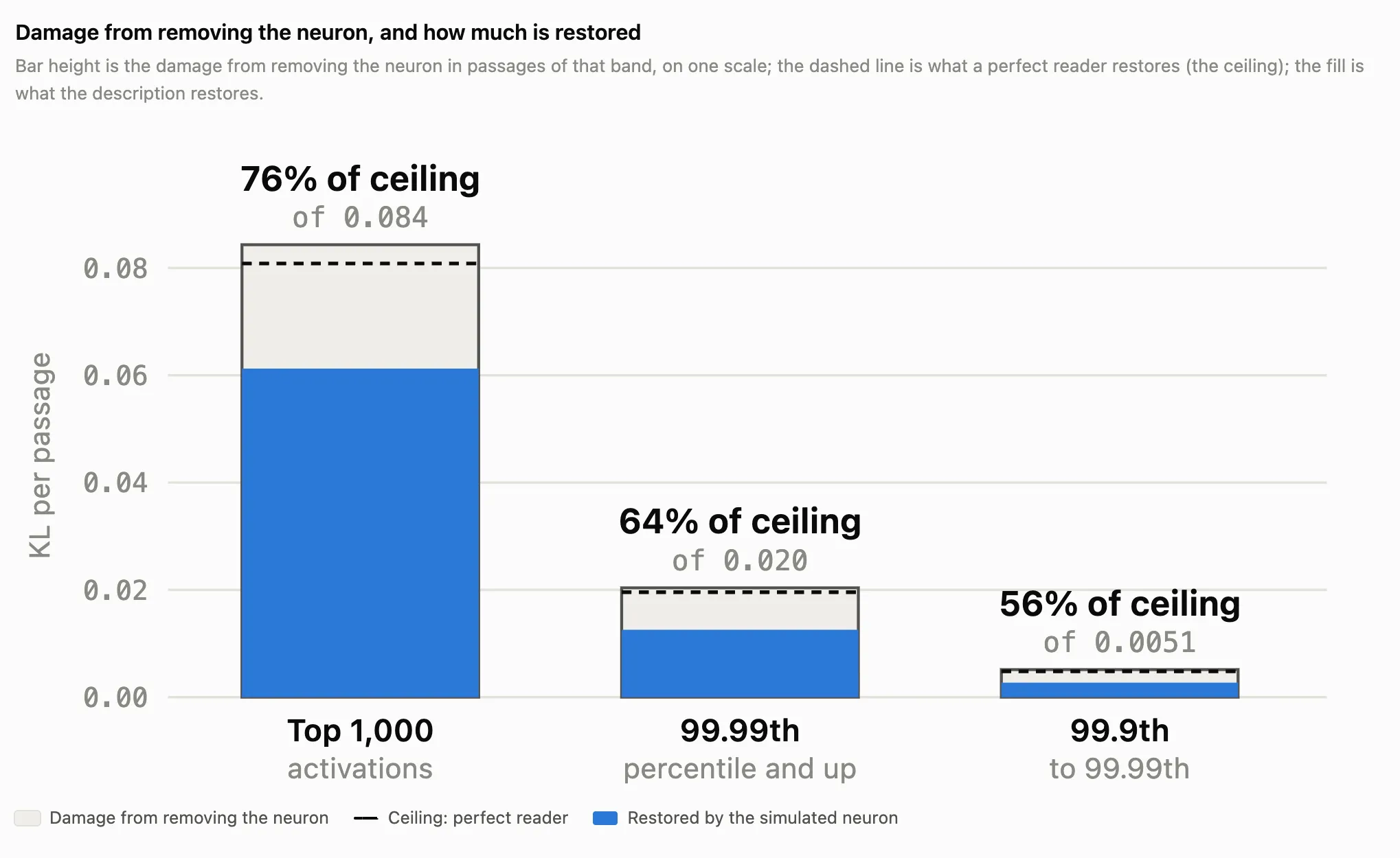
Passages, damage, simulator and ceiling
Passages. For each neuron, about 20 held-out passages per band (29,090 in all), each with one sampled activation from that band at token 45: the neuron’s 1,000 strongest router-weighted activations in a 10-billion-token corpus, activations at the 99.99th percentile and up, or activations from the 99.9th to 99.99th percentile. Negative poles use the corresponding negative tail. Passages often hold other firings too, and all of them are scored.
Damage. Change in next-word predictions (KL divergence summed over the passage) when the neuron is set to zero on every word piece routed to its expert on the pole’s side, gate open or closed. Restored = damage minus the change that remains with the simulated activation in place. Shares are ratios of means over neurons, so neurons that do more damage count for more.
Simulator. A reader model (Jev) gives a probability for each level 0–9 at every word piece from the neuron scientist’s description alone; the expected level is rounded, and a per-neuron table fitted on separate documents turns the level into an activation, with no constant or floor. Nothing inside the model is read.
Ceiling. A perfect reader that, at every word piece, picks whichever of the 10 levels the same table maps closest to the true activation. It restores 96% of the damage overall (95–97% by band); percentages above the bars are the simulator’s share of it.
Figure 12: Damage from removing a neuron and the share restored by its simulated activation across the three strongest activation bands. Percentages are relative to a perfect reader with the same 10-level scale and activation table.
Given the high bar that simulation must fulfill, we find the level of simulatability we are able to attain quite significant.
Input Synthesis
A final way to verify our neuron descriptions is to determine whether the description serves as an effective seed for generating texts that cause a maximal neuron activation (Erhan et al., 2009; Olah et al., 2017; Nguyen et al., 2016b; Fel et al., 2023c; Poerner et al., 2018; Thompson et al., 2024; Simonyan et al., 2013; Yosinski et al., 2015; Geirhos et al., 2023; Ghiasi et al., 2022). We attempt this on a random set of 128 neurons in Qwen 3.6 35B-A3B, using Claude Opus and Fable agents to generate the constructed examples.
We implement this procedure as follows. We designate a controller agent, generally a model like Claude Opus 5.5, who directs a set of synthesizer agents. The synthesizer agents’ jobs are simply to construct sentences based on the rules that the controller provides them. The controller receives a description of the neuron; no examples are provided. Based on the description alone, the controller agent creates a set of rules for the synthesizer agents, which they use to create candidate sentences. These sentences are then tested against the actual model to see if they cause the neuron to activate. The results are fed back to the controller agent, which then creates a new set of rules for the synthesizers to generate an improved set of candidates. This is repeated for several rounds until it reaches parity with or exceeds the natural corpus skyline, or until the maximum number of rounds is exceeded.
For each neuron, we measure how many rounds it takes to exceed the maximum activation value found in the natural corpus of 10B tokens, and how strongly we are able to make the neuron fire. Intuitively, a better description should result in faster convergence to a maximally exciting text.
Texts written from descriptions exceed natural activation maxima
Scroll horizontally to see all rounds.
This procedure succeeds in exceeding the natural corpus’ maximum 94% of the time. Though this method does not evaluate our ability to capture all of the different activation modes of a neuron, it does demonstrate that we are able to capture a strong sense of what the neuron responds to in its most causal modes through our descriptions.
We show some examples of the generated texts below.
- 1.55× }'echo "Disk:"df -h | awk 'NR>1 {printf "%s %s\n", $5, $6}'echo "Inodes:"df -i | awk 'NR>1 {print $5,
L24_E240_N188−In code, the name or index of a specific field, column or element being selected out of a data record.
- 1.46× t Agatha had sent Bertie down for a week to stay with Lady Pennyquick and her cousin LadyMid
L39_E115_N154−The start of a proper name, especially an unpredictable or invented one.
- 1.26× 'Sudha Pratibha Nandakumar, 78, of Chennai, passed away peacefully on March 3.
L24_E106_N379−The subword «and» in a South Asian given name or surname starting "Nand-".
- 1.19× y, and on Saturday the dentist found two more cavities. And it keeps going: problems uponproblemsupon problems upon problems. I am so tired.
L14_E218_N292−Rhetorical expressions of excess or overwhelming quantity: things piling up, one after another, too many to count or list.
- 1.04× Μπανγκόκ, Τζακάρτα, Μανίλα, Σιγκαπούρη και ηΚουάλα Λουμπούρ— κάθε μία συμβάλλει με τον δικό της τρόπο στην οικονομική και
L36_E144_N46+Kuala Lumpur, Malaysia, as an upcoming or current place name.
- 1.03× Why?!! Now I will never reallyknow.
L24_E132_N259+A future or modal clause claiming that a specific open question will never be answered.
- 1.02× tes in coal mines and is historically called firedamp, the miners' old name for it? Answer:methane, which seeps from coal seams and has caused countless mining explosions when igni
L39_E79_N331+Methane and other alkane (-ane) hydrocarbon names. The neuron fires at the point where such a name is about to appear.
- 1.02× ,老橡树上有什么东西咕咕、咕咕、咕咕地叫个不停,黑暗中闪着两只圆圆的眼睛——是貓头鹰。
L36_E137_N183+The opening piece of a multi-token bird name.
All 128 neuron poles
- 1.55× }'echo "Disk:"df -h | awk 'NR>1 {printf "%s %s\n", $5, $6}'echo "Inodes:"df -i | awk 'NR>1 {print $5,
- 1.46× t Agatha had sent Bertie down for a week to stay with Lady Pennyquick and her cousin LadyMid
- 1.43× 和页边距。喜欢竖排阅读体验的用户也可以尝试静读天下、超星阅读器或多看阅读,三者对繁体竖排小说支持较好。
- 1.41× want to achieve, and we design a plan that fits you. Because the plan is yours alone, youonlypay for the sessions you actually need, and nothing is padded out to fill a term.
- 1.39× se resp) throws ServletException, IOException {String scheme;scheme=hreq.getScheme();resp.getWriter().println("ok");}```
- 1.34× 1971United Arab Emirates | 1971 | 1971By 1971, all five Gulf states discussed in this chapter—Kuwait, Qatar, Oman, Bahrain and the Un
- 1.32× 任何风险由用户自行承担。四、本软件更新内容及版本号信息可能存在滞后,本站概不保证该等信息之准确性,具体以软件内置的“检查更新”功能为准。五、本站不提供数据备份、系统恢复等售后服务
- 1.31× A 25-watt bulb emits about 250 lm. A 40-watt bulb emits about4
- 1.29× La rotazione (scorrimento circolare) è un'operazione sui bit di una parola:ilbit che esce da un lato rientra dall'altro lato, a differenza dello scorrimento logico do
- 1.29× out departing from the scope of the invention, and the invention contemplates all obviousvariations, modifications and equivalents of the structures and methods described herein.
- 1.26× 'Sudha Pratibha Nandakumar, 78, of Chennai, passed away peacefully on March 3.
- 1.25× ttributions were computed using the Captum library, treatment effects were estimated withtheEconML package, and the identifying assumptions were validated via the DoWhy toolkit.
- 1.23× n sich selbst hat: das Gefühl, wertvoll zu sein und Respekt zu verdienen. Menschen wollensichals Teil einer Gruppe fühlen und von anderen akzeptiert werden.
- 1.22× r masses.Problem 1. Fresh nickel powder reacts with carbon monoxide gas to form Ni(CO)4. What mass of Ni(CO)4 is produced from 25.0 g of nickel, assuming excess
- 1.22× .Brooks, F. P. (1995). Ten pounds in a five-pound sack: Reports onsoftwareengineering (Anniversary ed.). Addison-Wesley.Cook, R. D. (1977). Detection
- 1.20× 陶然亭公园。石评梅的代表作有《涛语》《偶然草》等,散文集《石评梅选集》于1980年代重新出版。今天,山西平定县建有石评梅纪念馆。
- 1.20× learning to align and translate," in Proc. ICLR, 2015.[11] H.Sak, F. de Chaumont Quitry, T. Sainath, and K. Rao, "Acoustic modelling with
- 1.19× 列车实施超速防护;当列车实际速度超过允许速度时,系统自动施加紧急制动。司机通过司机室显示屏(DMI)查看列车当前速度、允许速度和目标距离。第十三条 列车进站前,司机应确认站台屏蔽门
- 1.19× Worked solution. Expand everything. Use the right-hand side e^xexpandedabout x=0, namely 1 + x + x^2/2.
- 1.19× y, and on Saturday the dentist found two more cavities. And it keeps going: problems uponproblemsupon problems upon problems. I am so tired.
- 1.18× N) vừa công bố báo cáo về tự do tôn giáo trên thế giới, cho thấy hàng triệu Kitô hữu đangbịbách hại vì đức tin. Tại nhiều quốc gia, các tín hữu bị bắt bớ, nhà thờ bị đóng cửa và
- 1.18× over the period.The change in Arizona's population is explained by three components:natural increase (the surplus of births over deaths), net international migration, and ne
- 1.18× s of the observations.6. r measures the strength of a linear relationship.7. r doesnotchange when we change the units of measurement of x, y, or both.
- 1.18× 忽見那女子躍身而起,劍鋒一轉,衣袖揚起如雲,剎那間,那白衣女子舞步躚然,宛若當年公孫大娘再現人間,滿座皆驚。
- 1.17× *w)3 2 2 2 2 2o7 = ideal (x - y*w,x y - z*w , x*y - z w)o7 : Ideal of R
- 1.17× arguments passed to the application.</param>public static void Main(string[] args){
- 1.16× on method for fuzzy system of linear equations, Applied Mathematics and Computation 163 (2005) 553-563.[3] S. Mitchell, R. Collins, A
- 1.16× import {Dividers} from 'antd';\nimport {Button} from 'antd';\n\nexport default () => <div><Dividers/><
- 1.16× helps the weekends. There is no mowing, no edging and no weekly fertiliser run.Soilimprovementinvolves what you cannot see. Deep roots open channels for water and air, and earthworms
- 1.16× 免责声明:本站部分内容来源于网络,如有侵权请联系删除。您的热心是对原创的最大支持。
- 1.15× Cử chỉ hùnghổcủa hắn khiến ai cũng sợ.
- 1.15× 2.10) Information about variantsVariants will be accepted: noII.2.10) InformationaboutvariantsVariants will be accepted: noII.2.13) Information about European Union fund
- 1.15× weak digestion. Ginger and bitter herbs are traditionally said to assist in the digestionoffood.
- 1.14× Excel recognizes as a date. The way this function interprets the string is controlled bytheregional settings in the Windows Control Panel. If the string is "6/9/2013", the function
- 1.14× 안경렌즈 하드코트 처리란, 표면에 하드코트를 도포하여 내스크래치성을 강화하는 표면 처리 공정을 말합니다. 일반 플라스틱 렌즈(CR-3
- 1.13× he 36 hours of the storm. The whole beach was cut back and lowered between the first cross-sectionand the last. We ran the first cross-section, at 06:00 on the morning of the first day
- 1.13× 主编:阎乐
- 1.12× Abbott, B. P., et al. (2017).‘GW170817: Observation of Gravitational Waves from a Binary Neutron Star Inspiral". Physica
- 1.12× Translation of: Snap!This task implements the classic Sieve of Eratosthenes usingSnap!, the visual, blocks-based programming language built on top of Scratch's design philosop
- 1.12× Problem A. Beautiful Array\n\nInput\nFirst line contains anumberT, the number of test cases.
- 1.12× sicionEntrePantallasDeConfiguracionAvanzada As Integer = ParametrosGenerales.ObtenerTiempoTransicionEntrePantallas()
- 1.12× Among the Egyptians, Thoth is ever representedunderthe form of a man bearing the crook and the flail, and his sister Isis appears beside him
- 1.11× Kaleler birer birer düşmüş, halk açlıktan kırılıyordu; tehlikeye giren saltanatınıkurtarmak için genç sultan ordusunu topladı.
- 1.11× C17. El 17 de julio de 2014, según la investigación, el vuelo MH17fue derribado.
- 1.11× From: Geoffrey R.Stone<gstone@uchicago.edu>\nTo: Faculty List\nSubject: Re: Workshop schedule\n\nDear colleague
- 1.10× onsider viscosity solutions of the fully nonlinear elliptic equation $$\mathcal{M}^{-}(D^{2}u) \le 0 \le \mathcal{M}^{+}(D^{2}u) \
- 1.10× d with curved hemostats to avoid the overlying intercostal vessels, and the subdermal airsacmembrane, thin, translucent and avascular, was penetrated bluntly.
- 1.08× vieron vuestros padres, cuando estuvieron al otro lado del río, o a los dioses de los amorreos en cuya tierra habitáis; pero yo y mi casa serviremos a Jehová. 16 Entonces el pueblo r
- 1.08× seconds:Mar 11 09:14:02 myservice[1234]: http:TLS handshake error from 10.0.0.17:51234: remote error: tls
- 1.07× Sichuan Province is home to the world-renownedgiant panda.
- 1.07× The first loaf was too salty and the second was bland. As for the choice of flour,I prefer a stone-ground whole wheat with a little rye blended in, because it holds moistu
- 1.07× 58, Delphos St. John's 52. Shelby County Athletic League: Fort Loramie 66, Russia 39; Botkins 52, Jackson Center 48; Anna 70, Fairl
- 1.07× Some reasons including heat,pressure and friction can cause the material to deform.
- 1.07× a game on an array of n integers (Rai and Joshi 2019). The judge, who keptcountof every even number Alice has taken, awards the win.
- 1.06× kgSolution: Recall what density is. Let us rebuild the formula from first principles.Density is a mass spread through a volume, so its units are those of mass divided by thos
- 1.06× The goal is to reverse that. A strengths coach does not ignore your weaknesses; she helpsyoumanage them, by delegating them, by partnering with someone whose strengths cover your ga
- 1.06× 铎与主教的共融,信友与牧者的共融,构成教会的合一。与罗马宗座的完全共融,是天主教会的标记。在圣体圣事中,我们彼此共融,与基督共融,与
- 1.06× $('#editor').keydown(function (evt) {if (!evt.originalEvent) {return;}if (evt.originalEvent.keyCode == 27) {
- 1.06× ilinoleoyl-sn-glycero-3-phosphoethanolamine;1,2-dilinoleoyl-sn-glycero-3-phosphoglycerol;1-linoleoyl-2-hydroxy-sn-glycero-3-phosphocholine.
- 1.06× e class — deductions Romney refuses to name.Then there are his numerous entitlementplans, which have evolved over eighteen months of campaigning. Which version he would actually
- 1.06× network programming from the Blue Network through the 1940s. In 1955 it switched to a"good music" and news format.
- 1.06× 이 책은 어려운 경제 이론을 초보자도 쉽게 이해할 수 있도록, 그림과 표를통해, 구체적인 예를 들어 친절하게 설명합니다.
- 1.06× nce for the financial sector is the subject of a new European framework. Regulation (EU) 2022/2554 of the European Parliament and of the Council on digital operational resilience fo
- 1.06× The two transportable strontium lattice clocks were moved by road tothelaboratory.
- 1.06× 2008年11月12日 網站改版上線 http://www.example.tw/•&2009年4月25日 新增RSS訂閱功能 http://www.example.tw/rss.xml•
- 1.05× with the validation values from the specification.selectp_brand,p_type,p_size,count(distinct ps_suppkey) as supplier_cntfrompartsupp,partwherep
- 1.05× fluorescent light hums and flickers. Is the problem more likely the tube, the starter orthe
- 1.05× о,точно този най-малко ми даде, как,и когато го питах какво ли,⏎той само се усмихна.
- 1.05× The word pachylobus appears in the index of Don's General History of the Dichlamydeous Plants. The word pac
- 1.05× gle fibre, lower the micropipette slowly into the muscle until a fibre is successfully impaled; a brief buzz of capacitance compensation helps the tip penetrate the membrane.
- 1.05× ;using System.Collections.Specialized;using System.ComponentModel.Design;using ZKWeb;using ZKWeb.Web;
- 1.05× .ndarray:"""Build the adjacency matrix of a graph.A set has no order, sowefirst convert the vertex set to a sorted list;the position of a vertex in that lis
- 1.05× $ is a perfect square they are rational. Also $\sqrt{\Delta} = 8$. We use $x = \frac{-b \pm \sqrt{\Delta}}{2a}$.
- 1.05× \n| 1 | Nick Drake | Pink Moon | Island | 1972 | Folk | [Spotify](https://open.spotify.com/album/1Czp6sYvO9Z1qVzHcfUfp
- 1.05× 电影《极速天使》由马楚成执导,汤唯、刘诗诗、韩彩英主演,讲述三位女赛车手的故事
- 1.04× [00:03.20] nama no koe de, kimi ni todoke[00:06.10] なまのこえで、きみにとどけ[00:09.00] nama no kimochi wo kakusanai de
- 1.04× ure- Fake Out- High Jump Kick- Zen Headbutt- Ice PunchSet details: FakeOutlets Medicham chip a lead and break Focus Sash, while High Jump Kick is the main STAB. Ze
- 1.04× but Gangwon had already completed the survey last month.[핵심 문장 번역]이들 지역 중 제주를제외한 나머지 지역은 이미 지난달 조사가 끝났다.
- 1.04× Μπανγκόκ, Τζακάρτα, Μανίλα, Σιγκαπούρη και ηΚουάλα Λουμπούρ— κάθε μία συμβάλλει με τον δικό της τρόπο στην οικονομική και
- 1.04× CAMBRIDGE, MA: MIT PRESS, 1961.12. P. M. SeNGE, The Fifth Discipline: The Art and Practice of the Learning Organization (New York: Doubl
- 1.04× Storage. A whole loaf keeps for four days. The bread, oncesliced
- 1.04× t me compare this with the given numbers. We computed the length PQ as 3 using the ratio.Butthe problem states that PQ is 2, so something is off. Let me go back to the similar trian
- 1.04× ers } from '../api/users';export function UserList() {const { data, isLoading,isFetching, error, refetch } = useQuery({queryKey: ['users'],queryFn: fetch
- 1.04× я Карамазовы. Книга первая.—Sí —dijo Zósima—. Hubo solo un par detalescasas en toda la provincia, y la segunda estaba abandonada desde la guerra.
- 1.04× world-class education to anyone, anywhere loading external resources on our website ( seeFigure1 )
- 1.03× corrosion inhibitor costcooling tower biocide costcooling tower chemicals bunnings⏎
- 1.03× measured versus predicted:Sample 1: measured 66,751, predicted 26,605.Sample 2: measured 41,208, predicted 38,915.
- 1.03× r the State Administrative Council and the ethnic armed organisations have agreed to signa
- 1.03× Why?!! Now I will never reallyknow.
- 1.03× 360;第三步:两边同时减去 72,消去常数项。2x = 288
- 1.03× with psychopy 2022.1.4 on macOS."""# PsychoPy importsfrom psychopyimport visual, core
- 1.03× 1313 = 13Because the statement is true, 5 is a solution.CHECK YOURSELF1Is 4 a solution of the equation 3x - 2 = 10?Two equations
- 1.03× quèrent dans le château. Le comte tenta donc de jeter des vivres et des gens d'armes danslaplace.
- 1.03× Testimonials from our students"Overall, I would say that, Professor Nguyendid
- 1.03× Better Business Bureau – Accredited BusinessesRoyal SEPTICandPlumbing1420 S. Peoria Ave – (918) 555-0142
- 1.03× ку на колени. Поезд трогается.Она закрывает глаза.* * *Когдаона открывает их, долины уже нет. Женщина напротив чистит апельсин. Запах наполняет вагон
- 1.02× tes in coal mines and is historically called firedamp, the miners' old name for it? Answer:methane, which seeps from coal seams and has caused countless mining explosions when igni
- 1.02× ,老橡树上有什么东西咕咕、咕咕、咕咕地叫个不停,黑暗中闪着两只圆圆的眼睛——是貓头鹰。
- 1.02× is delay, yet dared not press the matter, for it was the custom of that country that nonecouldsee the Khan save by his express command. At length, on the ninth day, a chamberlain of h
- 1.02× largest relations of their kind and are proved by exhibiting a suitable open bisimulationupto injective substitution.
- 1.02× Tilskotet vart auka i fjor.Tilsamanlikning fekk skulane mindre. Tiltaka skal evaluerast neste år.
- 1.02× zation. For every well, a z-score was calculated as the measured value of that particularwellminus the mean of all negative-control wells on the same plate, divided by the standard d
- 1.02× tember 2008. The Veteran has not alleged or demonstrated any prejudice with regard to thecontent
- 1.01× 49.== External links ==* Lecture by Smith on quantum optics, 1979, video intheRoyal Institution archive* John Smith at IMDb
- 1.01× pockets among the frankincense, are tapped in the same way. Their bark, when wounded, bleedsa dark reddish-brown resin that is noticeably stickier and slower to set.
- 1.01× the Carnegie foundation in 1912.In operations news, the second week found Abby thatshewas coming in early to help set up the new inventory tracking system, and her dedication
- 1.01× filter builder and the search syntax./// </summary>public interface IPredicate{string Name { get; }string Symbol { get; }bool Matches(object fieldValue,
- 1.01× 10月28日。本文来自于经济观察网
- 1.01× `sudo systemctl status nginx` || 开机自启 | `update-rc.d nginx defaults` | `sudosystemctl
- 1.01× with trade and manufacturing categories.1. Categories: Dead people | Fictional axeandhammer wielders | Knife and tool makers
- 1.01× insgesamt zwanzig Sekunden und wurde als Siebzehnter gewertet.Stand der Weltmeisterschaftnach dem Rennen
- 1.01× ,芙蓉楼即为其送别友人之处。洪江市东接溆浦县,南连会同县,西界
- 1.01× املا، وان الجانب الاميركي لن يقبل بتأجيل جديد. واشارت مصادر ديبلوماسية الى ان المسؤولينالاميركيين ابلغوا رئيس المجلس ان الوقت ينفد.
- 1.00× ght to be teaching others. Instead, you need someone to teach you all over again the veryelementarythings about God's word. You are like babies who need milk and cannot eat solid food. 13
- 1.00× 1867 at Lambeth Palace Chapel.Marriage.—On 19 June 1849,
- 1.00× You cannot at the same time serve Godandmammon.
- 1.00× Average Weather during JanuaryinTunis, Tunisia\nThe average minimum temperature is 8.0°C. The amount of rain is normal wi
- 1.00× Экстракт центеллы запускает и поддерживает выработкуколлагена.
- 1.00× RAPP (1925–1932), VOAPP (1928–1932),MAPP (1923–1932), VAPP (1920–1928
- 1.00× ntras?<|im_end|><|im_start|>assistantSenamiestis laikomas Vilniaus miesto centru, ocentras tęsiasi iki Gedimino prospekto.
- 0.94× states such as// 'loading', 'loaded', 'interactive' and 'complete'.if (newScript.readyState) {newScript.onreadystatechange = function () {if (newScript.readyState ==
- 0.89× her, at last, she noticed, the first thin snow settling on the shoulders of a few peoplestillhurrying home.
- 0.79× s not creation. It is the next best thing, and I am glad to have it.\begin{theorem}\label{thm:main}There are infinitely many prime numbers; that is, for every integer $N$ there
- 0.79× 了该镇的堤坝,迫使数千人在黑暗中撤离家园,许多人只穿着睡衣。 “都没有了,我们还剩下什么?”一位年轻的母亲说。
- 0.71× пити до бази даних, і схоже, що другий колбек спрацьовує раніше,ніж завершився перший. Через це в другому колбеку змінна result виявляється невизнач
- 0.68× Perfect!/// When thecurrentnode is visited, stop.
- 0.58× it. A family car tends to earn its keep more on the boring trips than on the exciting ones,
- 0.46× 【出版单位】 河北教育出版社【主办单位】 河北省教育厅【卷】 十【Volume】12
We consider this a useful validation of the primary mode of each neuron-pole, especially at the higher activation levels, though it does not validate the full range of functions that a neuron can compute.
How we interpret these results
We can synthesize maximally-activating texts across neurons, and predict neuron activations to a significant degree. At p99.9/0.1 and above, we are also able to recover 73% of the perfect-reader ceiling for the difficult task of per-token simulation on a neuron's highest activation bands. Though we see that there is still room to improve these simulation metrics, we can clearly see that increased amounts of intelligence and compute consistently increase our scores. Moreover, there may be a ceiling on what is predictable through text: the description must not only describe what the neuron is detecting from text, but must also to some degree anticipate the intermediate model computations, including attention, that lead to a neuron firing.
We find these results quite compelling nevertheless. Not only can we enumerate a neuron’s modes, but we can also describe its behavior to a meaningful extent! This is far from the expectation we started out with and we think it has strongly positive implications for the field of interpretability.
Example neuron descriptions
So what do the neurons we’ve analyzed look like? We find a vast landscape of fascinating structures among them, encompassing a broad range of computations. We see evidence of universal primitives, collections of convenient heuristics, dataset artifacts, and many more phenomena. Alongside this article we are releasing a dataset of circuit diagrams, activation examples, and Neuron Scientist-authored pages for each of the stratified set of 2,734 representative neurons in Qwen 3.6 35B-A3B. To provide some initial examples:
- Helping people live more independently (L13_E133_N30): Responds to writing about technology and support that help older or disabled people communicate, manage daily activities, or live independently. The surrounding context matters: the response brings together information about the kind of writing and the benefits being described.
- Trying a new approach after getting stuck (L16_E9_N229): Responds when a problem solver has tried something, failed, and tentatively proposes another approach: “Hmm, this isn’t working. Maybe I should try…”. The response often lands on “Maybe” or “Perhaps”. Looking back with regret, as in “Maybe I should have used…”, produces little response.
- Registering a moment of self-questioning (L9_E98_N330): Responds when the model interrupts its reasoning with “Wait”. Increasing its influence can then push the model to settle on an answer too quickly, including accepting a planted wrong answer; pushing it in the opposite direction encourages more self-questioning. Its effect fits a signal that doubt has already been raised.
- Crossing into the next month or year (L4_E190_N436): Responds when a date moves into the next month or year relative to an earlier date in the text. It responds at “June” in “31 May – 1 June”, or at the final digit of “2016” after a date in December 2015. The earlier date can be hundreds of word pieces away. Responses are strongest just after the calendar changes; repeating the same month or moving backwards produces little response.
- Marking a finding as estimated or uncertain (L14_E2_N240): In research writing, responds to words that qualify a result before naming it: “estimated risk”, “predicted pathways”, “possible interactions”, or “self-reported” measurements. Replacing these with words such as “measured”, “observed”, or “actual” removes the response. Word order also matters: “the software predicted…” produces little response.
- Locating a place within its former borders (L24_E230_N452): Responds to the country, empire, or region in a place description when that place used to belong there but no longer does. Examples include “Vilna, Poland” and “Monongalia County, Virginia”. The same country or state name produces little response when it still contains the place, as in “Krakow, Poland” or “Fairfax County, Virginia”.
- Keeping track of “release” elsewhere in a document (L36_E110_N224): Its strongest responses occur in documents mentioning “release”, across uses such as a release lever, a mould-release coating, a press release, or a software release date. The response may appear on a space, number, or punctuation mark away from the word itself. Looking only at the immediate phrase misses the connection.
- Comparing someone’s condition with their age (L24_E121_N186): Responds to descriptions such as “mature for her age”, “I’m 24 but look 16”, and “wise beyond her years”. The comparison must involve age and an age-related quality, such as maturity, appearance, or health. Replacing age with weight or cost removes the response.
Alongside this writing, we provide a library of neurons for browsing and also release the low-effort labels for all 10 million neuron-poles.
Conclusion
Implications for neuron interpretability
Analyzing neural networks in the neuron basis has often been treated as unworkable. In this view, neurons mix so many unrelated functions, or distribute meaningful computations so diffusely, that studying individual units offers little insight into how the model actually works. Our work stands in contrast to this view, adding to a growing body of work that finds neurons are more interpretable than previously thought. In the model and activation regimes we study, we can interpret most neurons as having one to a handful of computational roles. We can also trace their contributions through sparse circuits.
Alongside Arora et al. (2026), we find that sparse but strong activations are responsible for the majority of a neuron's causal effect. Removing the weakest activations preserves substantial model function, and brief fine-tuning recovers benchmark performance even with approximately 88% of routed neuron activations removed. Our circuit experiments reveal further sparsity: for specific functions, a handful of neurons per layer can reproduce the effects of the entire MLP layers they occupy. These findings allow us to focus our interpretive efforts on the high-activation regimes where neurons are both most consequential and most readily understood.
Within these regimes, most neuron poles have a single or a small number of coherent, computational roles. Even when neuron poles have multiple roles, we can concisely describe and distinguish them through their upstream inputs and downstream readers. Heterogeneity is less common than previously thought, and less problematic when it does arise: understanding a neuron’s different roles and how the models use them can provide a useful explanation of its computation.
Our agent, the Neuron Scientist, turns these explanations into testable predictions. Its descriptions are precise enough that a simulator can predict neuron activations from the description alone, recovering approximately 73% of the perfect-reader ceiling for KL damage from ablation in the strongest activation regime. These results show that concise descriptions can capture a substantial share of the causal effects of the neuron firings we study.
We approached this work believing that neurons resist direct study and that, as a result, neural networks require some sort of transformation or untangling before we can understand how they work. Instead, we found that models can operate under considerable neuron sparsity; that most neurons have one or a few coherent computational roles; and that we can describe those roles well enough to simulate their firings. We also found that scaling agent-driven investigations reliably improves our explanations. This gives us optimism that continued direct study, with better agents, tools, and methods, can yield significant advances in interpretability.
The ability to devote substantial compute to interpretability in general, and to understanding neurons in particular, is a major change in our field. Agents are now capable enough to conduct experiments, inspect circuits, and test hypotheses. This lets us conduct detailed investigations of individual neurons at a scale that would be near impossible to achieve manually. Scaling these investigations could yield superlinear gains: understanding more neurons provides upstream and downstream context, which we have already shown makes interpretation easier. We see substantial room to improve the agent harness, experimental tools, and simulation methods, and to measure how the resulting understanding scales with compute.
Future Work
Much about neurons remains to be understood. We still need to understand how neurons acquire their computational roles during training, how heterogeneous modes arise, and what weak and Q3 activations contribute. We must also establish how far these findings generalize across models and behaviors. But neurons already show substantial promise as a basis for understanding circuits, steering and probe vectors, and higher-level behaviors such as reasoning. The next step is to connect these increasingly precise accounts of individual neurons into explanations of the larger computations they jointly implement.
This work is our first technical post in a series on native interpretability: studying the original network via its own units, rather than via a replacement for them, as outlined in “Neural Networks Are Already Clean”. We are especially interested in a few directions for future research: new ways to zoom out from single neurons to the larger computations in which they take part while staying faithful to the network’s own mechanisms; how neurons and circuits form during training; and how attention and neurons work together.
For a more extensive discussion of open questions in neuron interpretability, and what remains to be explained, see the appendix.
Acknowledgements
We are grateful to our friends and colleagues who contributed to this work and provided feedback on early drafts. We would particularly like to thank Aryaman Arora, Leon Bergen, Usha Bhalla, Dan Braun, Lucius Bushnaq, Michael Jae Byun, Oliver Clive-Griffen, Fatih Dinc, William Dorrell, Matt Feiszli, Thomas Fel, Tucker Fross, Atticus Geiger, Tarun Gogineni, Tal Haklay, Dron Hazra, Eric Ho, Thomas Icard, David Klindt, Andrew Lee, Jack Lindsey, Ekdeep Singh Lubana, Jack Merullo, Lee Sharkey, and Connor Watts.
Author Contributions
Curt Tigges: Performed much of the research on the LLM side, including developing sparsification methods, creating methods for identifying subcircuits and modes, designing agents to do neuron research, and conducting wide-scale studies of neuron populations. Identified how neurons’ multiple meanings can be disambiguated downstream. Developed KL-recovery-based simulation and other evaluation methods. Studied thousands of neurons. Wrote much of the post.
Matthew Kowal: Helped run some of the additional experiments for the sparsity and simulation sections. Helped with writing and organizing the post. Studied 10s of neurons.
Thomas McGrath: Provided guidance and ideas for experiments and research directions, provided feedback for writing and early outlines.
Owen Lewis: Helped with project organization, writing, and the design of some experiments and metrics.
Nick Cammarata: Started the project in October 2025. Created the first neuron papers. Built the first agents for describing neurons and circuits. Developed the blind maximum technique and first polysemanticity score measures. Studied thousands of neurons. Improved simulations. Improved the total neuron view and built the mode profiles. Did the Colorado neuron studies and wrote that section. Designed the header. Had a minority role in writing and editing the text more broadly.
Appendix
Additional Results
Extended Sparsity Results and Discussion
Fine-tuning for performance recovery
We performed a brief fine-tuning protocol on the top-64 sparse model to see if we could recover performance. Our protocol used only 100M tokens (compared to the multiple trillions used to train the original model), and involved both SFT and RL:
- Start: the masked model. Qwen3.6-35B-A3B with a top-K mask, which keeps the top-K expert-neuron events per token (e.g., top-64 equates to ~12% of the expert’s neurons). We apply the same mask on the model during every training step and all weights are trained. SFT, as distillation: The student was trained to match the original model's next-token distributions, using a KL loss against the unmasked clean model as teacher. The data was the unmasked model's own thinking traces on prompts disjoint from every eval, plus 20 percent general web and reasoning text as anchors. We used 91M tokens of this dataset over 1,000 steps. This recovered about 72% of the drop in SuperGPQA, but showed a plateau after further SFT. We thus added RL.
- RL with verifiable rewards: Each round (a cycle of sampling followed by 10 training steps), the current model answered 1,024 knowledge prompts 4 times each: training-split multiple-choice and short-answer questions such as MMLU-auxiliary, MedMCQA and ARC. A sample scored 1 if it finished thinking and its answer matched the gold answer (an exact option letter, or an LLM judge for short answers). Each sample's advantage was its reward relative to its group. The loss was a policy gradient plus a small KL penalty (weight 0.1) toward the clean model, at learning rate 1e-6, 10 steps per round, for 10 rounds. Step 100 was the best checkpoint. It mainly taught the model to commit and stop in time: SuperGPQA reached 45.4 against clean's 44.8, with cap-hits below the original model’s.
Why finetune? When we observe rollouts directly, we see that the sparsified model’s reasoning tends to loop and self-check excessively. However, when we classified these rollouts with Claude Opus 5.5 agents, we identified that the sparsified model would still mention the facts and correct answers, usually as the last answer candidate–it would just self-check endlessly afterwards. We thus applied the finetuning in order to correct reasoning slip-ups, theorizing that the model might be calibrated to be sensitive to the statistics of the weak activations.
As a control, we also applied the same finetuning regime to bottom-448 (the complement of top-64) and random-64 models, where the filter only allowed those subsets of the neurons through. Fine-tuning the top-64 and layer top-320 models was successful.
As a result of this fine-tuning, we were able to bring the ablated model to parity and even beyond in some cases. Below are the benchmarks for the original, ablated, and fine-tuned models.
Benchmarks before and after fine-tuning
Accuracy change from the base model, in percentage points. Base-model scores are percentages.
| Benchmark | Baseline | Ablated, untrained | Trained under the mask (SFT → RL v1) | Reference: Top-64 | |||||||||
|---|---|---|---|---|---|---|---|---|---|---|---|---|---|
| Base model | Resample | Top-64Untrained | Top-320Untrained | Random-64†Untrained | Bottom-448†Untrained | Top-64†RL v1 | Top-320†RL v1 | Random-64†RL v1 | Bottom-448†RL v1 | Full model†RL v1 | Top-64RL v1 (orig.) | Top-64†RL v3 (RACE) | |
| Routed-expert cells ablated | — | 0% | 87.5% | 92.2% | 87.5% | 12.5% | 87.5% | 92.2% | 87.5% | 12.5% | 0% | 87.5% | 87.5% |
| Classic suiteLog-likelihood, greedy; GSM8K generated 5-shot | |||||||||||||
| ARC-Challenge · acc_norm | 54.7 | — | +3.6 (95% interval excludes zero) | +0.5 | −28.8 (95% interval excludes zero) | −32.8 (95% interval excludes zero) | +6.0 (95% interval excludes zero) | +2.0 (95% interval excludes zero) | −18.3 (95% interval excludes zero) | −23.1 (95% interval excludes zero) | +0.1 | +6.4 (95% interval excludes zero) | +5.7 (95% interval excludes zero) |
| ARC-Challenge · acc | 54.9 | — | +2.0 | +0.3 | −32.8 (95% interval excludes zero) | −37.3 (95% interval excludes zero) | +3.1 (95% interval excludes zero) | −0.5 | −22.5 (95% interval excludes zero) | −25.6 (95% interval excludes zero) | ±0.0 | +3.7 (95% interval excludes zero) | +2.9 (95% interval excludes zero) |
| ARC-Easy · acc_norm | 72.1 | — | +3.7 (95% interval excludes zero) | +1.9 (95% interval excludes zero) | −33.2 (95% interval excludes zero) | −41.1 (95% interval excludes zero) | +6.0 (95% interval excludes zero) | +2.8 (95% interval excludes zero) | −16.3 (95% interval excludes zero) | −19.4 (95% interval excludes zero) | +0.1 | +6.3 (95% interval excludes zero) | +6.4 (95% interval excludes zero) |
| ARC-Easy · acc | 81.4 | — | +0.8 | +0.2 | −40.3 (95% interval excludes zero) | −49.1 (95% interval excludes zero) | +2.0 (95% interval excludes zero) | +0.7 | −23.4 (95% interval excludes zero) | −26.3 (95% interval excludes zero) | +0.2 | +1.8 (95% interval excludes zero) | +1.9 (95% interval excludes zero) |
| WinoGrande · acc | 73.9 | — | −1.4 | −2.2 | −23.2 (95% interval excludes zero) | −23.6 (95% interval excludes zero) | −1.7 | −0.6 | −16.6 (95% interval excludes zero) | −15.9 (95% interval excludes zero) | ±0.0 | −1.3 | −1.6 |
| HellaSwag · acc_norm | 75.8 | — | −0.7 | −1.8 (95% interval excludes zero) | −35.2 (95% interval excludes zero) | −37.7 (95% interval excludes zero) | −2.2 (95% interval excludes zero) | −2.3 (95% interval excludes zero) | −23.7 (95% interval excludes zero) | −24.4 (95% interval excludes zero) | −0.2 | −1.7 (95% interval excludes zero) | −1.7 (95% interval excludes zero) |
| HellaSwag · acc | 57.4 | — | −0.7 | −1.6 (95% interval excludes zero) | −25.5 (95% interval excludes zero) | −26.9 (95% interval excludes zero) | −1.1 (95% interval excludes zero) | −1.2 (95% interval excludes zero) | −17.1 (95% interval excludes zero) | −20.4 (95% interval excludes zero) | −0.2 | −1.2 (95% interval excludes zero) | −1.1 (95% interval excludes zero) |
| MMLU · acc | 84.2 | — | −1.6 (95% interval excludes zero) | −1.2 (95% interval excludes zero) | −60.1 (95% interval excludes zero) | −60.9 (95% interval excludes zero) | −1.6 (95% interval excludes zero) | −1.0 (95% interval excludes zero) | −40.5 (95% interval excludes zero) | −49.8 (95% interval excludes zero) | +0.2 | −1.7 (95% interval excludes zero) | −1.1 (95% interval excludes zero) |
| GSM8K · strict | 96.7 | — | +0.3 | −1.7 | −96.3 (95% interval excludes zero) | −94.0 (95% interval excludes zero) | ±0.0 | −0.3 | −81.3 (95% interval excludes zero) | −73.7 (95% interval excludes zero) | +1.0 | −1.3 | −0.3 |
| GSM8K · flexible | 97.0 | — | +0.3 | −1.7 | −96.7 (95% interval excludes zero) | −94.3 (95% interval excludes zero) | −0.3 | −0.7 | −81.7 (95% interval excludes zero) | −73.3 (95% interval excludes zero) | +0.3 | −1.3 | −1.0 |
| Thinking panel4,096-token cap; a capped trace counts as wrong | |||||||||||||
| SuperGPQA | 44.8 | +2.6 | −15.2 (95% interval excludes zero) | −13.0 (95% interval excludes zero) | −44.5 (95% interval excludes zero) | −44.6 (95% interval excludes zero) | −0.5 | +0.2 | −32.5 (95% interval excludes zero) | −39.8 (95% interval excludes zero) | +5.1 (95% interval excludes zero) | +0.6 | +0.7 |
| MMLU-Redux | 91.5 | +1.0 | −3.7 (95% interval excludes zero) | −3.0 (95% interval excludes zero) | −89.0 (95% interval excludes zero) | −90.4 (95% interval excludes zero) | +1.9 (95% interval excludes zero) | +0.8 | −40.1 (95% interval excludes zero) | −73.2 (95% interval excludes zero) | +2.6 (95% interval excludes zero) | +2.0 (95% interval excludes zero) | +1.2 |
| MMLU-Pro | 78.4 | −1.1 | −8.5 (95% interval excludes zero) | −8.3 (95% interval excludes zero) | −78.0 (95% interval excludes zero) | −78.0 (95% interval excludes zero) | −1.4 | −2.9 (95% interval excludes zero) | −54.7 (95% interval excludes zero) | −74.0 (95% interval excludes zero) | +0.1 | −2.5 (95% interval excludes zero) | −3.4 (95% interval excludes zero) |
| IFEval | 30.9 | −0.6 | −0.6 | +0.4 | −15.9 (95% interval excludes zero) | −15.2 (95% interval excludes zero) | +0.2 | −1.1 | −3.1 (95% interval excludes zero) | −5.5 (95% interval excludes zero) | −0.6 | +0.2 | ±0.0 |
| Panel V2Thinking; raw, and on the items both arm and clean finished | |||||||||||||
| MedQA | 92.8 | +0.3 | −7.8 (95% interval excludes zero) | −4.6 (95% interval excludes zero) | −83.9 (95% interval excludes zero) | −80.6 (95% interval excludes zero) | −0.4 | −1.1 | −55.4 (95% interval excludes zero) | −81.2 (95% interval excludes zero) | +0.7 | −0.7 | −0.3 |
| MedQA · both finished | 95.9 | −0.1 | −1.8 (95% interval excludes zero) | −0.4 | −87.6 (95% interval excludes zero) | −83.5 (95% interval excludes zero) | −0.6 | −1.4 (95% interval excludes zero) | −47.3 (95% interval excludes zero) | −83.8 (95% interval excludes zero) | +0.4 | −0.4 | ±0.0 |
| GPQA-Diamond | 63.6 | −3.0 | −18.2 (95% interval excludes zero) | −11.1 (95% interval excludes zero) | −54.0 (95% interval excludes zero) | −55.6 (95% interval excludes zero) | +11.6 (95% interval excludes zero) | +2.0 | −44.9 (95% interval excludes zero) | −49.0 (95% interval excludes zero) | +9.1 (95% interval excludes zero) | +9.6 (95% interval excludes zero) | +6.6 |
| GPQA-Diamond · both finished | 88.3 | −3.4 | −2.5 | −1.1 | −78.5 (95% interval excludes zero) | −78.7 (95% interval excludes zero) | −1.5 | ±0.0 | −56.2 (95% interval excludes zero) | −67.0 (95% interval excludes zero) | −1.5 | −5.3 | −4.0 |
| MATH-500 | 69.8 | +0.8 | +7.0 (95% interval excludes zero) | +5.8 (95% interval excludes zero) | −69.8 (95% interval excludes zero) | −69.8 (95% interval excludes zero) | +0.6 | −0.4 | −65.6 (95% interval excludes zero) | −68.4 (95% interval excludes zero) | +2.8 (95% interval excludes zero) | −1.6 | +2.4 |
| MATH-500 · both finished | 99.1 | −0.6 | +0.6 | +0.6 | −98.9 (95% interval excludes zero) | −98.8 (95% interval excludes zero) | +0.9 | +0.6 | −69.0 (95% interval excludes zero) | −87.0 (95% interval excludes zero) | +0.6 | +0.3 | +0.9 |
| AIME 24+25 | 0.0 | +5.0 | +11.7 (95% interval excludes zero) | +11.7 (95% interval excludes zero) | ±0.0 | ±0.0 | +5.0 | +6.7 (95% interval excludes zero) | ±0.0 | ±0.0 | +1.7 | +8.3 (95% interval excludes zero) | +1.7 |
| AIME 24+25 · both finished | — | — | — | — | — | — | — | — | — | — | — | — | — |
| HumanEval+ | 59.1 | +0.6 | +7.9 (95% interval excludes zero) | +15.9 (95% interval excludes zero) | −59.1 (95% interval excludes zero) | −59.1 (95% interval excludes zero) | +21.3 (95% interval excludes zero) | +14.6 (95% interval excludes zero) | −54.3 (95% interval excludes zero) | −57.9 (95% interval excludes zero) | +3.7 | +17.1 (95% interval excludes zero) | +20.7 (95% interval excludes zero) |
| HumanEval+ · both finished | 85.8 | ±0.0 | ±0.0 | −0.9 | −85.5 (95% interval excludes zero) | −86.5 (95% interval excludes zero) | −0.9 | +1.9 | −78.0 (95% interval excludes zero) | −83.0 (95% interval excludes zero) | +1.0 | ±0.0 | +0.9 |
| MBPP+ | 71.7 | +3.7 | −20.4 (95% interval excludes zero) | −20.9 (95% interval excludes zero) | −71.7 (95% interval excludes zero) | −71.7 (95% interval excludes zero) | +13.0 (95% interval excludes zero) | −1.1 | −61.4 (95% interval excludes zero) | −66.7 (95% interval excludes zero) | +3.2 | ±0.0 | +8.2 (95% interval excludes zero) |
| MBPP+ · both finished | 95.8 | ±0.0 | ±0.0 | +0.6 | −95.7 (95% interval excludes zero) | −95.9 (95% interval excludes zero) | +1.1 | ±0.0 | −73.1 (95% interval excludes zero) | −83.6 (95% interval excludes zero) | +0.8 | ±0.0 | ±0.0 |
How to read the table and evaluation notes
Resample: base model with a new sampling seed (classic suite is greedy, so none). Top-64: only the 64 largest-|activation| cells per routed expert kept. Random-64: 64 of the 512 cells per routed-expert slot drawn uniformly at random for every token. Bottom-448: all but the 64 largest-|activation| cells kept.
Top-320: layer top-K. At every MoE layer, each token keeps the 320 routed-expert cells with the largest |activation| × routing weight, ranked across all eight routed experts (4,096 cells). This ablates 92.2% of routed cells; the shared expert is untouched. The trained column uses SFT (1,000 steps) followed by RL v1 (100 steps) under the same mask.
Full model: no mask; same recipe (SFT skipped, student = teacher). Trained columns: SFT distillation → RL v1 (100 steps) on RL pools with MMLU-aux + ARC replaced by RACE. Panel V2 “both finished” rows compare only items where both the arm and base model produced an answer (the base model finished no AIME item at the 16k cap).
† Measured on 8×H100; the Top-320 RL v1 classic suite was measured on H200. Reference: published Top-64 RL v1 (original pools, H200) and this sweep’s Top-64 RL v3. Intervals: paired bootstrap (generation; 10,000 resamples for Top-320), ±1.96 × paired SEM (classic).
Table 8: Benchmark scores before and after post-training the sparsified model. Red indicates an accuracy decrease; blue indicates an increase. Only changes whose 95% interval excludes zero are shaded. Zero and other results are white; a dash means no result.
What does this tell us? One concern is that we have simply produced a different model: one that is more sparse but that behaves differently from the original model. We believe that despite the fact that the model has been fine-tuned, this provides evidence for the importance of the high-activation regime for the following reasons:
- The fine-tuning process was quite modest. Recovery on benchmarks was achieved with only 100M tokens of training data, 9M of which was RL. In the RL step, the model was provided with only 34KB of reward information, as the model was not trained on the correct answers themselves. For perspective: Qwen was originally trained on 34T tokens. Performance recovery from other pruning methods (ShearedLLaMa, Minitron) required billions of tokens of training data.
- The information was present in untrained rollouts; the observed fine-tuning benefits were primarily conciseness and answer commitment. The original top-64 and layerwise top-320 models would output the correct answer but endlessly self-check. Accuracy between the models before and after finetuning in cases where the model did produce an answer stayed flat.
- Our controls demonstrate that the complement of top-64 is completely non-functional. Bottom-448 is not able to produce answers, and fine-tuning did not restore it.
- Examination of the most-changed neurons after fine-tuning reveals that the neurons are still functionally the same. We ran a token harvest on the model after training, obtaining example texts across percentiles. Semantically, the neurons retained their meanings.
Sparse neuron circuits
We observe even more sparsity than the results above through circuit analysis, an observation previously made by Arora & Wu (2025). A complementary approach obtains interpretable neuron-level circuits by training transformers with sparse weights (Gao et al., 2025). We see this from two primary types of experiments: sparsifying attribution graphs obtained via relevance patching (which we do for single steps of inference and then for continuous autoregressive generation); and also using community detection methods to find a small group of neurons that are both necessary and sufficient for various functions.
RelP circuits
We conduct relevance patching (with some modifications; see Appendix) for a wide range of prompts, obtaining attribution graphs containing hundreds of thousands of neurons, and gradually sparsify the graph in order to measure what percentage of neurons suffice to capture 90% of the logit difference between the top logit and the average vocabulary (Vig et al., 2020; Heimersheim & Nanda, 2024; Zhang & Nanda, 2024; Meng et al., 2022a; Mueller et al., 2024; Mueller et al., 2025; Pearl, 2001):
A few thousand neurons, 0.2 to 0.8 % of the active routed units, recover 90% of the margin. Random sets of the same size recover at most 0.02 and never restore the top-1. These neurons are almost always activating at their strong tails:
cell set (RelP rank) | in p10–p90 | beyond p1 / p99 | beyond p0.1 / p99.9 | median |act| |
|---|---|---|---|---|
top 100 | 1–6% | 82–91% | ~52% | 2.6–2.9 |
top 800 | 5–8% | 54–63% | ~24% | 0.9–1.3 |
top 3,200 | 13–18% | 37–44% | ~14% | 0.5–0.6 |
top 8,000 | 20–26% | 28–35% | ~10% | 0.34–0.42 |
uniform null | 80% | 2% | 0.2% | typical neuron's p90 ≈ 0.16 |
Table 9
Continuous generation under circuit sparsity
The RelP circuits above each explain a single token prediction. To see whether this sparsity holds for autoregressive generation, we generated text from ten prompts across five topics (factual continuations, a story, code, a chat-template reasoning trace and a memorized passage), and computed one RelP graph for every generated token (about 1000 total).
We then measure sparsity in two settings. In the first, we mean-ablate every neuron outside the kept set—at the current token and at every earlier token—so the kept neurons must also reconstruct whatever the earlier text contributed. In the second, the earlier tokens keep their real activations, as they would after a normal forward pass, and only the current token's neurons are kept or ablated.
Sparse neuron circuits across a generation
Qwen3.6-35B-A3B · ten generations. Each dot is one measured token. Neurons are kept in order of RelP attribution until at least 90% of the logit margin is recovered and the predicted token remains the top prediction.
Panels A–B of 6
A Neurons needed, whole text ablated
729 tokens. Dashed: 6,400 neurons, the single-answer-token reference (3–6K).
B Share of active neurons, whole text ablated
729 tokens. Dashed: 0.2% and 0.8%, the single-answer-token reference range.
C Neurons needed, current token ablated
730 tokens. Overall median: 519 of 163,840 active neurons; middle half: 119–2,075. Dashed: all 163,840 neurons. No quartile band is drawn.
D KL vs neurons kept, whole text ablated
None = every neuron ablated. Dashed: 6,400 neurons. Whole-text curves end at 25,600 neurons kept.
E KL vs neurons kept, current token ablated
None = every neuron ablated. Earlier tokens keep their real activations. Current-token curves end at 12,800 neurons kept.
F KL with only the needed neurons kept
Dashed medians: 0.019 nats for whole text and 0.016 for current token. The leftmost bin includes every value ≤ 10⁻⁵.
Methods and exact plot data
Only rows marked in_figure = 1 in the supplied data are shown: 730 tokens from ten texts, with context length at most 208. Weak-signal predictions are excluded (less than two logits of margin lost under full ablation, or the token remains top-ranked). One whole-text measurement is missing, giving 729 points in A/B and the whole-text histogram; C and the current-token histogram use 730.
There are 163,840 active routed neurons per token. Margin is the predicted token’s logit minus the vocabulary’s average logit. Margin recovered compares the kept-neuron margin with the fully ablated and original margins. The count search uses doubling and three bisection steps (approximately ±9% resolution).
D/E floor each KL measurement at 10⁻⁴ nats before computing medians. “None” is positioned at 27.5 on the logarithmic horizontal axis. F uses 24 logarithmic bins, four per decade from 10⁻⁵ to 10; values are clipped into that range. The dashed histogram medians use the original, unclipped values.
Download the exact plot data (JSON). Tables below display seven significant digits; the download retains the supplied summary precision and every plotted scatter point.
A. Neurons needed, whole text ablated
| Text length | Tokens / texts | Median | 25th percentile | 75th percentile |
|---|---|---|---|---|
| 1–32 | 135 / 9 | 27,917 | 18,102 | 58,361 |
| 33–64 | 215 / 10 | 111,668 | 55,834 | 254,571.5 |
| 65–96 | 121 / 10 | 121,775 | 78,961 | 265,593 |
| 97–128 | 84 / 4 | 187,802 | 121,775 | 352,224.5 |
| 129–160 | 82 / 5 | 289,631 | 148,091.8 | 567,242.8 |
| 161–192 | 67 / 4 | 344,431 | 151,368.5 | 751,210 |
| 193–208 | 25 / 4 | 531,185 | 289,631 | 893,344 |
B. Share of active neurons, whole text ablated
| Text length | Tokens / texts | Median (%) | 25th percentile | 75th percentile |
|---|---|---|---|---|
| 1–32 | 135 / 9 | 1.023429 | 0.5845313 | 1.631141 |
| 33–64 | 215 / 10 | 1.450143 | 0.7198732 | 2.801 |
| 65–96 | 121 / 10 | 1.046839 | 0.6332067 | 2.25229 |
| 97–128 | 84 / 4 | 1.062646 | 0.6752527 | 1.881319 |
| 129–160 | 82 / 5 | 1.354631 | 0.626421 | 2.350878 |
| 161–192 | 67 / 4 | 1.174436 | 0.5218886 | 2.62469 |
| 193–208 | 25 / 4 | 1.5587 | 0.9159416 | 2.646864 |
C. Neurons needed, current token ablated
| Text length | Tokens / texts | Median | 25th percentile | 75th percentile |
|---|---|---|---|---|
| 1–32 | 135 / 9 | 872 | 249 | 3,805 |
| 33–64 | 215 / 10 | 734 | 136.5 | 3,200 |
| 65–96 | 121 / 10 | 617 | 119 | 1,600 |
| 97–128 | 85 / 4 | 308 | 84 | 673 |
| 129–160 | 82 / 5 | 336 | 96.25 | 2,635.25 |
| 161–192 | 67 / 4 | 336 | 109 | 1,148 |
| 193–208 | 25 / 4 | 238 | 119 | 1,467 |
D. KL vs neurons kept, whole text ablated
| Neurons kept | under 32 tokens n=129 | 32–63 n=216 | 64–127 n=209 | 128–208 n=176 |
|---|---|---|---|---|
| None | 4.30274 | 4.872544 | 4.892343 | 5.000062 |
| 50 | 3.394675 | 3.660604 | 4.152394 | 3.909782 |
| 100 | 3.057923 | 3.373173 | 3.762759 | 3.517491 |
| 200 | 2.608309 | 3.110382 | 3.477049 | 3.234365 |
| 400 | 2.04026 | 2.745677 | 3.362782 | 2.822754 |
| 800 | 1.618873 | 2.296717 | 2.864502 | 2.505214 |
| 1,600 | 1.041499 | 1.749082 | 2.378909 | 2.24465 |
| 3,200 | 0.6453847 | 1.255513 | 1.842109 | 1.767386 |
| 6,400 | 0.3010152 | 0.7478843 | 1.260479 | 1.408452 |
| 12,800 | 0.1411609 | 0.3279115 | 0.7384518 | 1.056384 |
| 25,600 | 0.07371002 | 0.1649695 | 0.4049508 | 0.7955503 |
E. KL vs neurons kept, current token ablated
| Neurons kept | under 32 tokens n=129 | 32–63 n=216 | 64–127 n=209 | 128–208 n=176 |
|---|---|---|---|---|
| None | 0.6905828 | 0.5946631 | 0.9154095 | 0.6605841 |
| 50 | 0.1664906 | 0.09913591 | 0.1059898 | 0.1022723 |
| 100 | 0.131798 | 0.05935095 | 0.0742482 | 0.05905915 |
| 200 | 0.09924323 | 0.03723326 | 0.04803566 | 0.04042292 |
| 400 | 0.07705427 | 0.01922565 | 0.02237796 | 0.02906568 |
| 800 | 0.06032616 | 0.01512471 | 0.01756313 | 0.023811 |
| 1,600 | 0.04735442 | 0.00955051 | 0.0115736 | 0.02359346 |
| 3,200 | 0.03571446 | 0.004925947 | 0.01063378 | 0.0129501 |
| 6,400 | 0.02732095 | 0.003467737 | 0.005369483 | 0.009308547 |
| 12,800 | 0.01696113 | 0.002249019 | 0.004639292 | 0.006699116 |
F. KL with only the needed neurons kept
| KL bin (nats) | Whole text (n=729) | Current token (n=730) |
|---|---|---|
| Below 0.00001778279 (includes ≤10⁻⁵) | 6.447188% (47 tokens) | 9.863014% (72 tokens) |
| 0.00001778279–0.00003162278 | 1.371742% (10 tokens) | 2.191781% (16 tokens) |
| 0.00003162278–0.00005623413 | 2.057613% (15 tokens) | 2.328767% (17 tokens) |
| 0.00005623413–0.0001 | 3.155007% (23 tokens) | 3.150685% (23 tokens) |
| 0.0001–0.0001778279 | 1.646091% (12 tokens) | 3.424658% (25 tokens) |
| 0.0001778279–0.0003162278 | 3.292181% (24 tokens) | 2.60274% (19 tokens) |
| 0.0003162278–0.0005623413 | 4.526749% (33 tokens) | 3.287671% (24 tokens) |
| 0.0005623413–0.001 | 3.840878% (28 tokens) | 3.972603% (29 tokens) |
| 0.001–0.001778279 | 4.115226% (30 tokens) | 3.287671% (24 tokens) |
| 0.001778279–0.003162278 | 3.703704% (27 tokens) | 4.109589% (30 tokens) |
| 0.003162278–0.005623413 | 2.743484% (20 tokens) | 2.876712% (21 tokens) |
| 0.005623413–0.01 | 5.349794% (39 tokens) | 4.657534% (34 tokens) |
| 0.01–0.01778279 | 6.721536% (49 tokens) | 5.205479% (38 tokens) |
| 0.01778279–0.03162278 | 5.21262% (38 tokens) | 5.616438% (41 tokens) |
| 0.03162278–0.05623413 | 8.77915% (64 tokens) | 4.931507% (36 tokens) |
| 0.05623413–0.1 | 8.093278% (59 tokens) | 7.534247% (55 tokens) |
| 0.1–0.1778279 | 8.367627% (61 tokens) | 7.945205% (58 tokens) |
| 0.1778279–0.3162278 | 9.602195% (70 tokens) | 8.630137% (63 tokens) |
| 0.3162278–0.5623413 | 5.898491% (43 tokens) | 5.753425% (42 tokens) |
| 0.5623413–1 | 3.840878% (28 tokens) | 4.383562% (32 tokens) |
| 1–1.778279 | 1.097394% (8 tokens) | 3.287671% (24 tokens) |
| 1.778279–3.162278 | 0.1371742% (1 tokens) | 0.8219178% (6 tokens) |
| 3.162278–5.623413 | 0% (0 tokens) | 0.1369863% (1 tokens) |
| 5.623413–10 | 0% (0 tokens) | 0% (0 tokens) |
Figure 14: Sparse neuron circuits across a generation. Each point is one generated token from ten generated sequences. Whole text: neurons outside the kept set at the current and all earlier tokens are mean-ablated. Current token: only neurons outside the kept set at the current token are mean-ablated; earlier tokens keep their real activations. Median lines use 32-token windows with at least ten tokens from at least three texts; shaded bands show the middle half of tokens, not confidence intervals. A: Neurons that must be kept to recover 90% of the logit margin when every other neuron in the text, at the current token and all earlier tokens, is mean-ablated; the dashed line marks the single-answer-token result from the previous section. B: The same counts as a share of all active routed neurons in the text so far; dashed lines mark the 0.2–0.8% range for single answer tokens. C: Neurons that must be kept when only the current token's neurons are ablated and earlier tokens keep their real activations. D: KL divergence of the next-token distribution from the original as neurons are kept, with the whole text ablated, one line per range of text length ("none" = every neuron ablated); the dashed line marks 6,400 neurons. E: The same with only the current token ablated. F: Distribution of KL with only the needed neurons kept, for both settings.
When we ablate across the whole sequence, the number of neurons needed grows about linearly with the length of the text (Panel A). As a share of the active routed neurons in the text (Panel B), however, it holds roughly constant at about 1% (median 1.2%), not far from the 0.2 -- 0.8% we see for single answer tokens. When only the current token is ablated (Panel C), a median of ~520 neurons (0.3% of that token's routed units) recovers 90% of the margin, and this does not grow with the length of the text.
These sparse circuits also largely preserve the broader next-token distribution, despite being selected only to recover the target logit difference. A fixed neuron budget becomes less effective as texts get longer when ablating the whole sequence (Panel D), whereas ablating only the current token shows no comparable deterioration with context length (Panel E). Allowing each circuit enough neurons to recover 90% of the logit difference typically keeps the next-token distribution close to the original in both settings, although a minority of tokens show substantial deviations (Panel F).
In summary, when generating a token sequence, the model writes each new token with a few hundred neurons, leaning on what it already computed for the previous tokens. Only when we also ablate the earlier tokens does the required neuron count grow with length, because every earlier token's small circuit then has to be rebuilt too, which equates to about 1% of all the neurons that originally fired during generation.
Transcoder Evidence for Sparsity
Transcoders approximate MLP computations with sparse replacement features that support circuit analysis (Dunefsky et al., 2024). Further evidence for neurons as a sparse, interpretable basis comes from Shabalin & Piotrowski (2026), who find the following:
- Transcoder features tend to recapitulate neurons (with aligned encoder and decoder directions), and these are the only stable features across different transcoder training runs (Paulo & Belrose, 2025; Leask et al., 2025; Fel et al., 2025; Heap et al., 2025; Chanin et al., 2024; Kantamneni et al., 2025; Wu et al., 2025);
- Top-K MLPs perform better than transcoders (on KL divergence) at matched sparsity after model finetuning
They conclude, overall, that transcoder features add relatively little beyond what can be obtained from neurons.
We take this further and investigate the question: When transcoders learn additional features that are not neuron-aligned, what do these features represent? Using orthogonal matching pursuit (OMP) to determine what neurons explain the features (Pati et al., 1993; Mallat & Zhang, 1993; Olshausen & Field, 1997; Costa et al., 2025, O’Neill et al., 2025), we find that the remaining transcoder features usually end up representing sparse combinations of neurons. These are usually composed of 2-64 frequently co-firing neurons and include multiple types:
- Features where the encoder direction is a mixture of several neurons’ input directions, but where the decoder direction is aligned with the dominant neuron in the group
- Features where the encoder and decoder are both mixtures of neurons
Additional transcoder features appear to consist of recapitulation of earlier-layer neurons and overfit features for specific textual templates.
1What each feature is, by layer and width
One row per dictionary. Dead: share of all features with 0 fires in 10M positions. Class shares: percent of the features that fired (each row sums to 100). Neurons with a copy: share of the layer's 131,584 neurons that have at least one neuron-copy feature. Census over 10,000,463 positions (12,800 documents).
Neuron copy
- Encoder reads
- one neuron's input rows
- Decoder writes
- that same neuron's output column
What it is
The transcoder rediscovered a neuron. L36 f101570 = L36/E116/N363+, nutrient cycling (read 0.91, write 0.97).
Neuron + read-side condition
- Encoder reads
- that neuron's own input row first (98–99%), plus a correction from 10–60 other neurons' input rows
- Decoder writes
- one neuron's output column
What it is
The neuron's own trigger, narrowed by context: it writes exactly what the neuron writes, but only in part of the neuron's range. L36 f28546 writes like L36/E145/N226− (“th”/“st” after digits) but fires on century markers (“19th century”).
Coalition: neurons fire together
- Encoder reads
- one input slice from each of many neurons
- Decoder writes
- a sparse sum of 2–64 neurons' output columns, and those neurons fire with the feature
What it is
A group of neurons the model itself activates together, packaged as one feature. Mostly means what the neurons share (1b). L19 f37368 = summation-notation neuron + binomial-coefficient neuron → the number inside \binom.
Combination: neurons do not fire together
- Encoder reads
- as above
- Decoder writes
- a sparse sum of neuron outputs, but those neurons do not fire when the feature does
What it is
Matches neurons on paper only: the weights fit a sum of neurons, but the activity does not back it.
Combination: too rare to test
- Encoder reads
- as above
- Decoder writes
- a sparse sum of neuron outputs
What it is
Geometrically a coalition like the two rows above, but it fired fewer than 10 times on the 919k-position co-firing ladder, so whether its neurons fire with it could not be tested. Similar in size to the tested coalitions (1c).
No same-layer match
- Encoder reads
- nothing sparse
- Decoder writes
- nothing within 64 neurons reaches cosine 0.7
What it is
Explained in section 2: mostly echoes of other layers' neurons or fixed phrases.
Transcoder feature composition
234M training tokens
L41× 9.8%
Share of features that fire (%)
- Neuron copy
- 11.7%
- Neuron + read-side condition
- 31.1%
- Coalition: neurons fire together
- 17.5%
- Combination: neurons do not fire together
- 8.9%
- Combination: too rare to test
- 23.3%
- No same-layer match
- 7.5%
L42× 9.2%
Share of features that fire (%)
- Neuron copy
- 6.5%
- Neuron + read-side condition
- 26.6%
- Coalition: neurons fire together
- 18.6%
- Combination: neurons do not fire together
- 4.5%
- Combination: too rare to test
- 35.4%
- No same-layer match
- 8.3%
L91× 26.1%
Share of features that fire (%)
- Neuron copy
- 32.2%
- Neuron + read-side condition
- 30.1%
- Coalition: neurons fire together
- 16.7%
- Combination: neurons do not fire together
- 7.2%
- Combination: too rare to test
- 10.4%
- No same-layer match
- 3.5%
L92× 27.4%
Share of features that fire (%)
- Neuron copy
- 19.1%
- Neuron + read-side condition
- 27.9%
- Coalition: neurons fire together
- 17.6%
- Combination: neurons do not fire together
- 5.5%
- Combination: too rare to test
- 23.6%
- No same-layer match
- 6.4%
L141× 28.5%
Share of features that fire (%)
- Neuron copy
- 34.4%
- Neuron + read-side condition
- 27.0%
- Coalition: neurons fire together
- 15.7%
- Combination: neurons do not fire together
- 5.8%
- Combination: too rare to test
- 13.3%
- No same-layer match
- 3.9%
L142× 17.2%
Share of features that fire (%)
- Neuron copy
- 12.4%
- Neuron + read-side condition
- 32.3%
- Coalition: neurons fire together
- 16.4%
- Combination: neurons do not fire together
- 3.3%
- Combination: too rare to test
- 32.4%
- No same-layer match
- 3.2%
L191× 38.9%
Share of features that fire (%)
- Neuron copy
- 50.9%
- Neuron + read-side condition
- 16.0%
- Coalition: neurons fire together
- 14.3%
- Combination: neurons do not fire together
- 6.0%
- Combination: too rare to test
- 6.8%
- No same-layer match
- 6.0%
L192× 48.8%
Share of features that fire (%)
- Neuron copy
- 36.1%
- Neuron + read-side condition
- 16.0%
- Coalition: neurons fire together
- 17.5%
- Combination: neurons do not fire together
- 5.2%
- Combination: too rare to test
- 13.8%
- No same-layer match
- 11.4%
L241× 24.6%
Share of features that fire (%)
- Neuron copy
- 32.7%
- Neuron + read-side condition
- 23.7%
- Coalition: neurons fire together
- 12.4%
- Combination: neurons do not fire together
- 8.3%
- Combination: too rare to test
- 12.2%
- No same-layer match
- 10.6%
L242× 30.9%
Share of features that fire (%)
- Neuron copy
- 23.9%
- Neuron + read-side condition
- 22.2%
- Coalition: neurons fire together
- 11.9%
- Combination: neurons do not fire together
- 6.2%
- Combination: too rare to test
- 18.7%
- No same-layer match
- 17.0%
L301× 35.6%
Share of features that fire (%)
- Neuron copy
- 47.1%
- Neuron + read-side condition
- 13.5%
- Coalition: neurons fire together
- 14.4%
- Combination: neurons do not fire together
- 3.5%
- Combination: too rare to test
- 15.3%
- No same-layer match
- 6.2%
L302× 42.4%
Share of features that fire (%)
- Neuron copy
- 34.3%
- Neuron + read-side condition
- 14.3%
- Coalition: neurons fire together
- 17.5%
- Combination: neurons do not fire together
- 2.4%
- Combination: too rare to test
- 23.1%
- No same-layer match
- 8.3%
L361× 36.2%
Share of features that fire (%)
- Neuron copy
- 51.6%
- Neuron + read-side condition
- 21.7%
- Coalition: neurons fire together
- 15.4%
- Combination: neurons do not fire together
- 3.1%
- Combination: too rare to test
- 6.4%
- No same-layer match
- 1.8%
L391× 5.0%
Share of features that fire (%)
- Neuron copy
- 7.3%
- Neuron + read-side condition
- 13.5%
- Coalition: neurons fire together
- 27.3%
- Combination: neurons do not fire together
- 4.3%
- Combination: too rare to test
- 37.0%
- No same-layer match
- 10.6%
L392× 4.4%
Share of features that fire (%)
- Neuron copy
- 4.1%
- Neuron + read-side condition
- 9.2%
- Coalition: neurons fire together
- 20.6%
- Combination: neurons do not fire together
- 3.9%
- Combination: too rare to test
- 46.1%
- No same-layer match
- 16.0%
Layer 19 retrained on 1B tokens: the width ladder
L191× 49.1%
Share of features that fire (%)
- Neuron copy
- 68.2%
- Neuron + read-side condition
- 16.2%
- Coalition: neurons fire together
- 6.5%
- Combination: neurons do not fire together
- 3.3%
- Combination: too rare to test
- 4.8%
- No same-layer match
- 1.2%
L191×, neuron-initialized 51.4%
Share of features that fire (%)
- Neuron copy
- 71.9%
- Neuron + read-side condition
- 16.7%
- Coalition: neurons fire together
- 5.5%
- Combination: neurons do not fire together
- 2.8%
- Combination: too rare to test
- 2.4%
- No same-layer match
- 0.7%
L194× 59.6%
Share of features that fire (%)
- Neuron copy
- 33.4%
- Neuron + read-side condition
- 18.8%
- Coalition: neurons fire together
- 15.6%
- Combination: neurons do not fire together
- 2.3%
- Combination: too rare to test
- 27.1%
- No same-layer match
- 2.9%
L198×, neuron-initialized 38.4%
Share of features that fire (%)
- Neuron copy
- 16.2%
- Neuron + read-side condition
- 23.5%
- Coalition: neurons fire together
- 10.9%
- Combination: neurons do not fire together
- 1.2%
- Combination: too rare to test
- 46.2%
- No same-layer match
- 1.9%
Table 10: Transcoder feature composition.
Coalitions mostly mean what their neurons share at every layer judged, and the share does not fall with size (60% at 2 neurons, 64% at 33–64). Combinations whose neurons do not fire together read as sets or as emergent three times as often (40% vs 12%), so co-firing is what separates a conjunction from a mixture.
1cHow many neurons a coalition combines
For every coalition feature whose neurons fire with it: the number of neuron output columns in its decoder's sparse sum (orthogonal matching pursuit, stopped at cosine 0.7, capped at 64), by dictionary. Last column: the same for the combinations too rare to test. On the read side, encoders need more rows: at L36, 67% of coalition encoders are rebuilt from at most 64 raw input rows and 33% need more than 64 (the random-direction null crosses 0.7 at about 80).
234M training tokens
L41× 21
Neurons in the coalition: share of coalitions (%)
- 2 neurons
- 13%
- 3–4 neurons
- 9%
- 5–8 neurons
- 9%
- 9–16 neurons
- 13%
- 17–32 neurons
- 20%
- 33–64 neurons
- 36%
L42× 25
Neurons in the coalition: share of coalitions (%)
- 2 neurons
- 10%
- 3–4 neurons
- 8%
- 5–8 neurons
- 9%
- 9–16 neurons
- 12%
- 17–32 neurons
- 20%
- 33–64 neurons
- 41%
L91× 21
Neurons in the coalition: share of coalitions (%)
- 2 neurons
- 12%
- 3–4 neurons
- 9%
- 5–8 neurons
- 9%
- 9–16 neurons
- 14%
- 17–32 neurons
- 24%
- 33–64 neurons
- 33%
L92× 26
Neurons in the coalition: share of coalitions (%)
- 2 neurons
- 9%
- 3–4 neurons
- 7%
- 5–8 neurons
- 8%
- 9–16 neurons
- 12%
- 17–32 neurons
- 23%
- 33–64 neurons
- 41%
L141× 26
Neurons in the coalition: share of coalitions (%)
- 2 neurons
- 9%
- 3–4 neurons
- 7%
- 5–8 neurons
- 8%
- 9–16 neurons
- 12%
- 17–32 neurons
- 22%
- 33–64 neurons
- 41%
L142× 25
Neurons in the coalition: share of coalitions (%)
- 2 neurons
- 8%
- 3–4 neurons
- 7%
- 5–8 neurons
- 8%
- 9–16 neurons
- 13%
- 17–32 neurons
- 24%
- 33–64 neurons
- 39%
L191× 22
Neurons in the coalition: share of coalitions (%)
- 2 neurons
- 12%
- 3–4 neurons
- 8%
- 5–8 neurons
- 9%
- 9–16 neurons
- 13%
- 17–32 neurons
- 20%
- 33–64 neurons
- 37%
L192× 30
Neurons in the coalition: share of coalitions (%)
- 2 neurons
- 8%
- 3–4 neurons
- 7%
- 5–8 neurons
- 7%
- 9–16 neurons
- 11%
- 17–32 neurons
- 20%
- 33–64 neurons
- 47%
L241× 25
Neurons in the coalition: share of coalitions (%)
- 2 neurons
- 10%
- 3–4 neurons
- 7%
- 5–8 neurons
- 8%
- 9–16 neurons
- 13%
- 17–32 neurons
- 22%
- 33–64 neurons
- 40%
L242× 30
Neurons in the coalition: share of coalitions (%)
- 2 neurons
- 8%
- 3–4 neurons
- 6%
- 5–8 neurons
- 7%
- 9–16 neurons
- 10%
- 17–32 neurons
- 21%
- 33–64 neurons
- 47%
L301× 23
Neurons in the coalition: share of coalitions (%)
- 2 neurons
- 11%
- 3–4 neurons
- 8%
- 5–8 neurons
- 9%
- 9–16 neurons
- 13%
- 17–32 neurons
- 20%
- 33–64 neurons
- 39%
L302× 30
Neurons in the coalition: share of coalitions (%)
- 2 neurons
- 8%
- 3–4 neurons
- 6%
- 5–8 neurons
- 7%
- 9–16 neurons
- 11%
- 17–32 neurons
- 21%
- 33–64 neurons
- 47%
L361× 8
Neurons in the coalition: share of coalitions (%)
- 2 neurons
- 22%
- 3–4 neurons
- 15%
- 5–8 neurons
- 13%
- 9–16 neurons
- 13%
- 17–32 neurons
- 16%
- 33–64 neurons
- 21%
L391× 14
Neurons in the coalition: share of coalitions (%)
- 2 neurons
- 11%
- 3–4 neurons
- 11%
- 5–8 neurons
- 14%
- 9–16 neurons
- 21%
- 17–32 neurons
- 27%
- 33–64 neurons
- 17%
L392× 14
Neurons in the coalition: share of coalitions (%)
- 2 neurons
- 10%
- 3–4 neurons
- 10%
- 5–8 neurons
- 14%
- 9–16 neurons
- 21%
- 17–32 neurons
- 27%
- 33–64 neurons
- 18%
Layer 19 retrained on 1B tokens: the width ladder
L191× 20
Neurons in the coalition: share of coalitions (%)
- 2 neurons
- 12%
- 3–4 neurons
- 10%
- 5–8 neurons
- 10%
- 9–16 neurons
- 13%
- 17–32 neurons
- 19%
- 33–64 neurons
- 36%
L191×, neuron-initialized 16
Neurons in the coalition: share of coalitions (%)
- 2 neurons
- 15%
- 3–4 neurons
- 12%
- 5–8 neurons
- 10%
- 9–16 neurons
- 14%
- 17–32 neurons
- 18%
- 33–64 neurons
- 31%
L194× 34
Neurons in the coalition: share of coalitions (%)
- 2 neurons
- 6%
- 3–4 neurons
- 5%
- 5–8 neurons
- 6%
- 9–16 neurons
- 10%
- 17–32 neurons
- 20%
- 33–64 neurons
- 52%
L198×, neuron-initialized 28
Neurons in the coalition: share of coalitions (%)
- 2 neurons
- 8%
- 3–4 neurons
- 7%
- 5–8 neurons
- 8%
- 9–16 neurons
- 12%
- 17–32 neurons
- 22%
- 33–64 neurons
- 44%
Coalitions span the whole range from 2 to 64 neurons; the median coalition combines 8–34 neurons depending on the dictionary, and 2× dictionaries usually make larger ones. The combinations too rare to test are of similar size (median 7–28), so they look like coalitions that seldom fire rather than a separate kind of feature.
Figure 16: Neuron coalitions by size.
When we examine transcoder features that consist of sparse combinations of neurons, we find that the transcoder feature represents a semantic combination or intersection of the neurons it is related to, rather than novel unrelated features. This suggests that, to the extent that there are features carried by multiple neurons, they are computed through composition (Olah, 2023; Mu & Andreas, 2020; Smolensky, 1990; Braun et al., 2025; Bushnaq et al., 2025; Braun et al., 2024).
Examples: features next to their neurons
Descriptions are short summaries. Feature descriptions are the exemplar gloss where one was written (coalition, echo and template rows), otherwise the dictionary label. Weights are the decoder’s sparse-combination coefficients; the sign picks the neuron’s pole (+ positive, − negative). Echo and template rows come from the layer-19 dictionary of section 2.
| Kind | Transcoder feature | Constituent neurons (weight) |
|---|---|---|
| Neuron copy | L36 f101570 Discussions of nutrient cycling, recycling, and reuse in ecological/agricultural contexts read cos 0.91 · write cos 0.97 | L36/E116/N363+ Nutrient cycling, decomposition, and recycling of organic matter in ecosystems, with terms like bacteria, nutrient, organic, decompose. |
| Neuron + condition | L36 f92499 Permutation formula and reasoning about selecting/arranging distinct items (P(n, r) = n!/(n-r)!) read cos 0.42 · write cos 0.87 | L36/E72/N477+ Combinatorial and algebraic formulas using variables n, k, c, r with fractions, exponents, summations, combinations, permutations, factorials, ratios, series. |
| Neuron + condition | L36 f28546 Ordinal century references like "17th", "19th", "20th" marking historical centuries or time periods read cos 0.41 · write cos 0.83 | L36/E145/N226− Ordinal suffixes "th" and "st" after digits in century references, like "19th century" and "21st century". |
| Coalition: intersection | L19 f37368 Numeric digits in binomial coefficient arguments, like the top slot of \binom{1}{7}, C(n-1, m), C_{23}^{5}, C(4,2). 2 neurons in total | L19/E54/N375+ +0.60 Mathematical expressions with summations, subscripted variables, superscripts, and LaTeX notation like ∑_{k=1}^n, parentheses, and brackets. L19/E54/N168+ +0.55 Binomial coefficients and combinatorial notation like "C(n, k)" and "n choose k", with variables n, k, r, x, plus "coefficients", "sorted", "frequency". |
| Coalition: intersection | L36 f7323 Nouns for measurable attributes (diet, size, habitat, morphology, mineral) used to distinguish or categorize entities, including organisms and minerals. 2 neurons in total | L36/E116/N377− −0.65 Measurable traits like size, color, mass, or diet analyzed or compared in biological, ecological, experimental contexts, with "distribution," "abundance," "variation," "classification" L36/E116/N13− −0.57 Distinguishing or confusing similar species by color, wing markings, tail features, size, seasonal plumage; hybridization, separation, identification traits. |
| Coalition: intersection | L9 f69927 Words for leaders or leadership of political, military, or organizational bodies ("leader," "led," Spanish "lider," Punjabi "agvai"), plus linking prepositions like "of" 3 neurons in total | L9/E33/N395+ +0.57 Internal structure of communist and revolutionary movements: sections, chapters, groups, affiliations, and integration within international organizations, historical parties, labor movements, ideological factions. L9/E33/N406− −0.31 The word "leading" meaning a key or prominent role, as in "leading part in," "leading member of," "leading figures," "leading theatres" L9/E33/N426− −0.21 Mentions of "Central Committee" (or its translations) as a governing body within parties, governments, or institutions, especially in roles and decisions. |
| Coalition: set (any of) | L36 f111164 The word "grand"/"Grand" in any sense: grand jury, Grand Duke, Grand Prix, grandstand, grand opening, Grandey, grandiflora. 2 neurons in total | L36/E148/N198− −0.66 The word "grand" in legal terms like "grand jury" and indictment, and in psychology like grandiose, inflated self-image. L36/E148/N127+ +0.40 "Grand Duke" and "Grand Duchess" noble titles in historical or genealogical texts, with places, dates, family relationships. |
| Echo | L19 f26 Token "Crest" in "Family Crest Products" headings on genealogy pages with surnames, notables, migration dates. | L14/E219/N15− Heraldry and noble genealogy: coats of arms, crests, bends, armorial bearings, heralds, family branches, titles, cognomen. |
| Echo | L19 f3530 The word "opposite" in geometry problems, like "sides a, b, c opposite angles A, B, C respectively" in triangle ABC. | L47/E77/N122− Triangle ABC sides a, b, c paired with opposite angles A, B, C, via the phrase "opposite to". |
| Echo | L19 f1456 Code-golf challenge rules stating that the shortest entry wins: "code-golf", "fewest bytes wins", "lowest byte-count", "shortest". | L9/E137/N294+ Code golf and optimization: minimizing code length or data size, text processing, with words like "characters," "bits," "saved," "shortest," "golf" |
| Template | L19 f3791 Download notice telling users to ensure they have an application to open this file type before downloading or purchasing. | no same-layer neuron expresses it; a fixed phrase recurs across its examples |
| Template | L19 f11026 Quirky author-bio blurbs ending scraped blog posts, like "Zombie enthusiast. Subtly charming travel practitioner. Webaholic" | no same-layer neuron expresses it; a fixed phrase recurs across its examples |
Table 11: Examples of semantic composition. Multiple types of composition occur here, and we also show the neuron-copy features along with the neuron feature modulated by a condition.
Neuron coalitions usually consist of groups within the same expert, and we find that the mixed features’ labels generally track the dominant neuron in the group or represent a semantic intersection of those neurons.
Although this does not rule out features spread diffusely across many neurons, the features recovered by transcoders support a picture in which individual neurons are meaningful units of computation, and concepts without a dedicated neuron are represented through combinations of neurons.
Additional Analyses of Modality Profiles
Neuron-pole profiles
Loading neuron-pole profiles…
How to read these profiles
Height runs from weak, common firings to strong, rare firings. Width is average KL damage per firing, compressed using a fourth-root scale so weak firings remain visible. Areas are not damage shares; the printed percentages give frequency-weighted damage shares among assigned modes.
Blue marks the dominant group of linked modes, lighter blue a possible link, and other colors groups with no link seen. Gray is reserved for firings assigned to no mode. Gate-closed firings (negative gate inputs, Q3/Q4) are excluded.
The group boundaries and prevalence estimates are approximate. They use 991 sampled poles, excluding 50 without sufficient gate-open data. Some single-mode examples stand in for others; the displayed shares sum to about 100%.
The browsable selection omits 87 poles flagged for explicit content or interpretation concerns; these remain in the prevalence estimates. Mode labels and link judgments are provisional.
Additional subcircuit and mode comparisons
There is much more similarity between subcircuits in a mode vs. subcircuits between different modes:
| Top-50 overlap per pair | Within a mode | Between modes | Ratio | Neurons where within beats between |
|---|---|---|---|---|
| Inputs | 9.8% | 2.0% | 4.9× | 96% |
| Readers | 9.9% | 3.1% | 3.2× | 95% |
Table 12
We also see that modes are highly identifiable by the set of neurons reading the target neuron at a given activation, even at the lower percentile bands:
| Band | Readers, mode | Chance |
|---|---|---|
| q95 | 0.76 | 0.33 |
| q99 | 0.79 | 0.33 |
| q99.9 | 0.84 | 0.31 |
| q99.99 | 0.88 | 0.35 |
| extreme 1,000 | 0.95 | 0.48 |
Table 13
Example neuron modes
Democratization / making resources accessible to everyone rather than an elite
KL per firing1.3× avg
Read description and 10 subcircuits
Text about broadening access to something formerly exclusive or costly (art, knowledge, technology, AI models, finance, luxury, education, therapy) so that it is available to all. This covers normative claims ('Art for all', 'knowledge should be free'), mission statements ('make X available/accessible to all', Robinhood's 'Democratize finance for all'), open-sourcing and democratization of LLMs, cheap democratized luxury and fashion, 'within everyone's reach' idioms across languages, and the outward dissemination or sharing of ideas, information and resources to many recipients. Firing falls on the access, open, reach or democratize keyword, the universal-audience phrase ('for everyone', 'à la portée de tous'), or the predicate slot after the claim is set up.
- c8 Widening access/availability of services to broader audiences (democratize access) 21.0%
- c7 Robinhood 'Democratize finance for all' slogan; democratizing access 14.6%
- c1 Normative endorsement that knowledge/art/technology should be accessible to all 12.3%
- c2 Democratization: art/culture made accessible to everyone, not elites 6.6%
- c3 Anticipating 'make X available/accessible to all' in mission statements 5.4%
- c4 Openness / open-sourcing of AI models and technology access 4.6%
- c5 Open access to knowledge as a universal right 4.4%
- c6 Democratization of luxury: costly goods made affordable to everyone 2.3%
- c9 Spreading/sharing ideas, news, viruses outward to many ('spread the', 'share') 1.3%
- c10 'within everyone's reach' accessibility/affordability idioms across languages 0.6%
Subcircuit bars are scaled to the largest share shown.
Inserting, attaching or coupling an instrument into or onto a receiving target (needles, catheters and tubes into the body; probes, chucks and connectors onto vessels and devices)
KL per firing1.3× avg
Read description and 13 subcircuits
The pole fires at the moment a penetrating or coupling instrument reaches its target, whether that target is a body or a piece of apparatus. On the medical and bodily side this covers hypodermic needles entering ports or the spinal cord (c10), intubation and tubes passed into the trachea or stomach (c8), rectal probes and enema tips (c9), microelectrodes impaling a cell (c6), and an inhaler mouthpiece placed between the lips (c7). It also covers ophthalmic instruments inserted into or applied to the eye (c12) and needles or objects inserted into a body in sexual or medical-fetish scenes (c13). On the mechanical side it covers filling or vent needles and probes inserted into or sealed against containers (c1), electrical test probes contacting a device under test (c2), plugs and connectors hooked up to terminals or cylinders (c3), and pump chucks placed on tire or shock valves (c4). It further covers teat cups attached to a cow's udder in milking equipment (c5) and parts brought into mating engagement, such as a pinion meshing with a ring gear (c11). Every case is the same situation: an instrument is put into, onto or against a target structure, usually with the peak on the target or on the completion of the insertion.
- c10 Access needles inserted into ports, cord, or vessels 18.4%
- c1 Filling/leak-test probe or needle inserted into, sealed against vessel 17.6%
- c2 Electrical test probes contacting device under test (meters, wafer pads) 7.0%
- c3 Equipment hookup points: battery terminals, couplers, cylinder hookups 5.0%
- c13 Forced needle/catheter/object insertion into body in sexual-fetish scenes 4.2%
- c4 Pump head/air chuck coupling onto tire or bike valve 4.1%
- c6 'Impale' = microelectrode penetration of cells in intracellular recording 3.9%
- c7 Inhaler instructions: placing mouthpiece in mouth / between lips 3.7%
- c5 Milking machinery: teat-cup attachment, milking parlors and stalls 3.6%
- c8 Intubation: inserting a tube or catheter into the trachea or rectum 2.6%
- c9 Rectal insertion of enema tips, probes and colonic tubes 2.0%
- c12 Instrument-accessed target: eye fundus in ophthalmic devices, tree tap-holes 1.4%
- c11 Mechanical parts brought into mating engagement (gears, wrenches, threads) 1.1%
Subcircuit bars are scaled to the largest share shown.
Figure 18: Two modes (of two different neurons), each of which contains a rich cluster of related subcircuits. Each “c” prefix shows a subcircuit label, and percentages on the right indicate how much of the neuron’s firing is performed by the subcircuit on our dataset.
Random Baselines for Neuron Circuits
A handful of neurons does what hundreds of random directions do
Specific neurons are wired to specific neurons; random directions are not
Subcircuits and meanings change with firing strength
Figures 19–21: Random baselines vs. neuron phenomenology. Figure 19: recovery of ablation function for sparse selections of neurons vs. random directions, selected on a greedy basis. Figure 20: selectivity of reader neurons for neurons vs. random directions. Figure 21: differences in subcircuit and mode distribution through the activation range of a neuron vs. random baselines.
A Colorado neuron with a rare Tornado mode
We examine the most popular counterexample we could find to Neural Networks Are Already Clean: a Colorado neuron in Qwen3-32B (L55/N11703) that also fires on code using Tornado, a Python web framework (Brangus, 2026).
About 98.8% of the neuron's causal effect comes from text about Colorado, other mountainous places, or other locations, decreasing as places become less Colorado-like. Much of this text is only subtly about Colorado: a citation of Lynne Rienner Publishers, which is based in Boulder; a review of South Park; a quote from a researcher whose CU affiliation appeared 150 tokens earlier. For each ambiguous case, we ablated tokens one at a time and traced the circuit driving the activation, rather than judging relatedness from the text alone. In the remaining 1.2%, no single input strongly activates or suppresses the neuron; its activation is composed from thousands of small positive and negative contributions.
Colorado’s share of effect: 56%
- Place names24%
- Schools15%
- Companies6.0%
- Teams6.5%
- Media2.4%
- People0.07%
- Other1.9%
Figure 22: From firing to causal effect.
The Tornado association is causally real. Asked which state Tornado was developed in, Qwen3-32B assigns 30% to Colorado and 0.7% to the correct answer, California (Brangus, 2026). Suppressing the neuron reduces Colorado to 1% and raises California to 4.7%. The neuron's meaning alone predicts this error.
Tornado is not one of a large set of hidden secondary functions. Across 100 million tokens of ordinary text, the neuron fired at ≥30% of its typical Colorado peak 3,812 times. Of these firings, 98.5% were on Colorado or other places, Tornado appeared three times within a single document, and the remaining 1.4% formed 18 small groups of one or two documents each. On a code corpus, 98% of strong firings were on Tornado or code that calls it.
The two computations interact very little. Tornado predictions run mostly through code and web-library neurons. The Colorado neuron appears in 6.6% of their attribution graphs, and zeroing it costs 0.005 nats per token, a twelfth of the cost of Tornado's own top detector. Among the roughly 200 neurons that contribute to predicting Colorado, 94% of sampled firings reflected those neurons' primary functions, and none of the remainder involved code. Colorado and Tornado route 2% of their relevance through shared neurons, comparable to what Colorado shares with unrelated web libraries.
Across the broader circuits behind Colorado and Tornado framework related content, both run mostly through neurons performing their primary functions, with about 5% of firings appearing unrelated. This estimate fell with each closer inspection (from an initial 10–16%), because subtle relationships are difficult to identify across hundreds of neurons, so we treat it as probably higher than the true amount with substantial uncertainty. The unrelated firings are dispersed across many neurons rather than sharing a common theme. The one recurring overlap is Tornado itself: because layers 32–55 appear to copy layers 8–31, the pathway in which Tornado neurons feed a Colorado neuron at layer 14 recurs at layers 37–38.
Colorado and Tornado
Neuron circuits across layers 0–63Colorado
827 predictions
- Half the push
- 155 neurons
- 80% of the push
- 2,299 neurons
Tornado
1,496 predictions
- Half the push
- 1,276 neurons
- 80% of the push
- 6,965 neurons
→ a Colorado name
- Colorado-specific29%
- Places in general28%
- Used for any word8%
- Rarely used neurons35%
23,789 neurons, each in under 2% of predictions. Most are doing their own job on another word in the passage: ‘Senate’, ‘summer’, a mountain name.
→ a Tornado identifier
- Tornado-specific10%
- Web libraries in general14%
- Used for any word8%
- Rarely used neurons68%
31,440 neurons, each in under 2% of predictions. Most are doing their own job on another part of the code: ‘import’, ‘Optional’, error handling.
Scroll horizontally to see the full figure.
Figure 23: Interactive Colorado–Tornado map.
We do not know why the Tornado association exists. We suspect Qwen3-32B was initialized by copying layers of Qwen3-14B, since many neurons align semantically 24 layers apart. One hypothesis is that the association served a minor sequence-level function in the earlier copy, such as continuing the second token of a certain kind of sequence, as in the layer 11 neuron. Copied into the more semantic later layers, the association may have been reinforced by appearing in both places rather than trained away. Without Qwen's training data or checkpoints we cannot observe it forming; future studies will focus on models where both are available.
We consider this a benign form of overlap. The two modes are easy to identify and separate: clustering the neuron's firings by their upstream inputs separates Colorado from Tornado perfectly, and the two computations meet only in a narrow pathway around layer 14 and its copy. Tornado also has its own representation among code neurons, so an analysis starting there would reach the overlap quickly. Full separation would be cleaner, but the overlap is narrow and traceable. Studying the original network also has an advantage here: a replacement basis that split Colorado from Tornado would lose the association that predicts the model's error. Because the modes are easily separable, analysis can move between the two views as needed.
Methods: Subcircuit and Mode Methods
Finding Neuron Subcircuits
To identify subcircuits, we group different firings of the same neuron according to which upstream inputs produce them, then use downstream effects to help decide which groups belong together. We collected firing examples by running 10 billion tokens from diverse domains through Qwen 3.6 35B-A3B, including data from pretraining, reasoning, chats with users, and math. For each of the model's 5 million neurons, we collected 1,000 examples from each of 14 activation percentile bands, for a total of 14,000 examples per neuron. We then collected an additional 30,000 examples per neuron for a stratified subset of 2,734 neurons. These additional examples were drawn from above the 95th activation percentile (p95) for positive poles and below the 5th percentile (p5) for negative poles. As a starting point for neuron descriptions, we used an internal version of Qwen3-8B that we fine-tuned to produce basic labels for each neuron based on example sentences the neuron fires on.
Setup. Consider a target neuron in routed expert of layer . At token position , with residual stream , its activation is
where and are the gate and up pre-activations. We call each projection a lane. A firing is one example from the neuron's examples; we write for the set of firings of one pole of .
Input attributions. To identify subcircuits, the first step is to characterize each firing by the upstream inputs that produce it. For each firing, we use first-order Taylor attribution to find the input neurons most responsible for the target neuron's activation (see Binder et al., 2016 for related Taylor-based attribution methods). We linearize the RMSNorm at its actual scale, . Each pre-activation then decomposes exactly into contributions from upstream components , whose writes to the residual stream are :
Many inputs contribute strongly to many neurons in the expert, rather than specifically to the target neuron, so we measure each input against the expert's average neuron. Let be the mean of over the 512 neurons of expert . For each lane we keep the 400 inputs with the largest excess .
Four-part profile. Let be the sign of lane 's pre-activation at the firing. We split each kept input's contribution into the part that supports this sign and the part that opposes it, each net of the expert baseline:
where . This gives each firing a profile with four parts: gate drivers , gate suppressors , up drivers , and up suppressors . Keeping these separate lets us distinguish firings where the same input plays different roles.
Readers. To collect downstream readers, we take the target neuron's write at the firing, , where is the router weight. We compute its first-order effect on the activation of every neuron in later layers at the same position, again through each reader layer's linearized RMSNorm. We keep the 1,000 readers with the largest ; for the last layer, the readers are output logits.
Weighting. We next compare these profiles across firings of the same neuron to identify upstream subcircuits that recur in different contexts. Inputs that appear in nearly every firing provide little information about what distinguishes one firing from another. We therefore weight each block with TF-IDF over the neuron's firings and then L2-normalize it:
where is the number of firings in which input appears. The four normalized blocks are concatenated so that each contributes equally:
The factor normalizes to unit length when all four blocks are non-empty.
Community detection. Since we do not know in advance how many subcircuits a neuron has, we use community detection to find groups of firings with similar input profiles. We split firings by document: 75% of documents form the fitting set , and the remaining 25% are held out for evaluation. We build a graph on the fitting set by connecting each firing to its nearest neighbors by cosine similarity, with edge weights
The graph is made undirected by summing reciprocal edges. We then run the Leiden algorithm (Traag et al., 2019) to find the partition that maximizes the Reichardt–Bornholdt configuration objective (Reichardt & Bornholdt, 2006) at resolution :
Here is the weighted degree of and is the total edge weight. Communities with fewer than 15 fitting firings are left unassigned. Each held-out firing is assigned to the community whose centroid is nearest in cosine similarity.
Merging. This procedure can split a single circuit into several groups. To bring these back together, we describe each group by two sets of 50 neurons:
-
Its top 50 input neurons , by mean TF-IDF driver weight and over its firings.
-
Its top 50 readers , by mean TF-IDF reader weight.
We link two groups when both overlaps reach a threshold :
The final subcircuits are the connected components of this link graph. Requiring agreement on both inputs and readers helps ensure that merged groups reflect the same underlying circuit.
This yielded a median of 19 subcircuits per pole (with a range between 1 and 51), with low overlap in their inputs and readers. We send each subcircuit, with a description of its inputs and readers, to Claude Opus 5.5 to produce a concise description of the subcircuit.
Modes
Claude Opus 5.5 produces three descriptions of each subcircuit:
- A semantic reading of the content the neuron tracks, based only on the text of six firings.
- A token-pattern description, based on the same six firings.
- A functional description, based on short labels for the most selective inputs and readers, in the form “combines X and Y to signal Z, used by readers that do W.”
The semantic reading receives no circuit evidence, allowing us to compare it with that evidence later. Readings must identify specific content rather than token form. Descriptions broad enough to fit a random neuron are rewritten.
We group subcircuits into modes in two Opus passes. The first groups subcircuits with the same meaning and classifies the pole as monosemantic if one specific underlying meaning accounts for all identifiable meanings, or polysemantic otherwise.
The second pass reviews the groups using longer contexts. Opus receives each mode’s label, subcircuit readings, KL damage, overlap with other modes, and up to three full-length exemplars. It first looks for document-level context that could connect the modes, then judges whether each pair reflects one mechanism or two. We applied this review to all 826 multi-mode poles in the random sample and used the resulting groups as our reported modes.
We measure the effective number of modes using the inverse Simpson index:
Reproducibility and simulation
We also checked whether the groupings were stable across repeated runs and different fitting documents. We repeated the Opus grouping three times on the first 219 poles. The runs agreed on whether a pole had one mode or several 96% of the time, with a median adjusted Rand index of 0.95. Clustering two halves of the fitting documents separately recovered 68% of subcircuits, compared with 1% under a shuffled null.
Methods: Evaluation Methods
We evaluate neuron descriptions at three levels: (i) detecting text that makes a pole fire, (ii) classifying the mode or subcircuit responsible for a firing, and (iii) simulating token-level activations well enough to reproduce the neuron’s effect on the model.
Data splits and exclusions
We use the document splits and activation bands described in the preceding section. Descriptions, subcircuit centroids, and retrieved examples use only the discovery and validation folds and we evaluate on a separate held-out test set.
To check for repeated contexts across folds, we compare the 16-token sequence ending at each firing and the 13-token sequence beginning at it. We count two contexts as repeated if either sequence matches exactly. Approximately 2.6% of firings repeat a context. Removing test-set firings whose context also appears in a fitting fold changes the headline results by at most 0.002.
Each pole also has a firing threshold, θ, which defines the activation unit used in simulation. For the pole included in the census, θ is the census threshold. For the opposite pole, θ is 0.65 times that pole’s own p99.9.
Detection setup
The detection task tests whether the mode descriptions help a judge distinguish text containing a held-out firing from a control sequence in which the neuron stays below q90.
Each firing sequence contains the sampled firing token, the 60 preceding tokens, and the eight following tokens. We construct two types of control sequences with the same window: same-expert controls use a token routed to the neuron’s expert, while random controls use a randomly selected corpus position. The sampled token is unmarked, so the judge is not shown the location of the firing. We randomize the order of the firing sequence and its control.
For this evaluation, we use the mode descriptions produced before the long-context review, excluding residue and gate-closed groups from the list shown to the judge. Each mode is presented with its label and description, along with up to three examples from the fitting data in which the firing token is marked.
The judge evaluates pairs of sequences in batches of 10, selecting the sequence containing the firing and reporting its confidence in each choice. We calculate accuracy separately for each pole within each activation band, then report the median across poles.
Description variants and context limits
To understand what limits detection performance, we test whether more detailed descriptions or combinations of text methods help, and examine whether the short sequences preserve the context that makes the neuron fire.
Adding more detail to the descriptions made little difference on a 40-pole development benchmark. The mode list alone achieved a detection AUROC of 0.909. Including each subcircuit’s label, semantic reading, and token pattern gave 0.914; adding examples from the fitting folds gave 0.911.
On 40 fresh poles, an ensemble of text methods reached a detection AUROC of 0.938. The “ensemble” combined Opus predictions from descriptions, Opus predictions from 10 retrieved fitting examples, refined descriptions, and an embedding classifier. It was evaluated against same-expert controls, with an AUROC of 0.838 at q95.
Alternatively, we found that shorter sequences can omit context that determines whether the neuron fires. When we rerun the underlying model on the sequence alone, approximately 15% of exemplars stop firing, while some controls begin firing. Providing 250 tokens of actual preceding context improves detection against same-expert controls:
The short sequence alone gives an AUROC of 0.927; adding 250 preceding tokens gives 0.978.
With the additional context, AUROC reaches 0.943 at q95. These results measure the underlying model’s behavior when rerun with different amounts of context; the text judge receives only the short sequence.
Reader-based classification
The classification task tests whether we can identify which mode was active by looking at how a firing affects downstream neurons.
For each firing, we retain the 1,000 downstream readers with the largest absolute attribution values. We represent the firing as a TF-IDF vector over these readers and normalize it to unit length.
We compute each subcircuit’s centroid from its fitting-fold firings. To classify a held-out firing, we calculate its cosine similarity to every centroid and apply a softmax with temperature 0.05. Each mode receives the highest score among its subcircuits, and we predict the mode with the highest score.
Readers are excluded from the initial clustering features but are used when merging clusters, using only fitting-fold firings. The evaluation therefore tests whether groups initially defined by their inputs also have distinct downstream effects, while retaining some dependence on readers during fitting.
The main classification evaluation includes only firings assigned to real modes. We exclude layer 39, which has no downstream routed readers, and test-set firings whose context also appears in a fitting fold.
We calculate two metrics separately for each activation band:
- Accuracy: the median fraction of correct predictions across poles. For mode classification, the baseline always predicts the pole’s most frequent mode. For subcircuit classification, chance accuracy is the sum of squared subcircuit proportions.
- Separation: each mode’s one-versus-rest AUROC, summarized as the median across pole–mode pairs. This measures whether the mode scores its own firings above other modes’ firings, even when it does not receive the highest score overall. Chance AUROC is 0.50.
Additional classification tests
On the 40-pole benchmarks, Opus receives the mode descriptions, eight retrieved fitting examples, and a test sequence. At q95, marking the firing token brings its accuracy close to the reader classifier’s, although readers achieve better separation between modes.
With the firing token marked, Opus achieves 0.825 accuracy and 0.944 separation AUROC at q95, compared with 0.824 and 0.973 for the reader-based classifier. Without marking the firing token, Opus reaches 0.74 accuracy.
We also test a stricter setting in which residue and gate-closed groups compete as possible answers. Assigning a real-mode firing to either group counts as an error. For text classification in this setting, Jev receives subcircuit readings and two examples per subcircuit, with the firing token unmarked in the test sequence.
Reader-based accuracy ranges from 0.78 at q95 to 0.96 in the extreme band for modes, and from 0.66 to 0.86 for subcircuits. Jev’s mode accuracy ranges from 0.40 to 0.83, compared with chance baselines of 0.36 and 0.60.
Under this stricter evaluation, both reader-based and text classification improve for stronger firings.
Token-level simulation
Simulation is a much harder test of our understanding of a neuron than detection or classification, requiring us to predict the neuron’s activation at every token accurately enough to reproduce its effect on the model. To do this, we get Claude Sonnet 5.5 to convert each description into a fixed JSON format describing what makes the pole fire, its token pattern, and its activation levels. Jev (jev-1.14) uses this description to assign each token a probability distribution over 10 activation levels, with level 0 representing silence.
We express activations relative to a threshold, , using the census threshold for the pole included in the census and 0.65 times the opposite pole’s own p99.9 for that pole. To convert the predicted levels into activations on this scale, we fit a separate monotone, non-negative calibration map for each pole using windows from the description side of the split. We select the ridge regularization strength through five-fold cross-validation, grouping windows by document so that windows from the same document remain in the same fold.
Each evaluation window contains the focal token, 45 preceding tokens, and 12 following tokens, preceded by another 768 tokens of actual context. During these runs, we keep routing fixed to the clean model’s routing and replace the neuron’s activation at all tokens with either the predicted value for simulation or zero for ablation.
Recovery score
For each window, we sum the divergence between the clean and patched next-token distributions, then compare the weighted totals for simulation and ablation:
Here, denotes simulation or ablation, is the next-token distribution at position in window , and is that window’s sampling weight. A recovery score of 1 means simulation reproduces the clean model’s predictions; 0 means it performs as well as removing the neuron, and a negative score means it performs worse.
We report both an unweighted average across poles and an average weighted by each pole’s ablation damage. The former describes performance on the average pole; the latter measures the fraction of aggregate ablation damage recovered.
Evaluation windows
All evaluation windows are held out from the description writer. We use three sampling schemes:
-
Activation bands: 20 windows per band—S95, S99, S99.9, S99.99, and Top—centered on sampled firings. Top contains the pole’s 1,000 strongest firings. We either weight the bands equally or weight them by the proportion of routed tokens in their activation intervals.
-
Threshold-relative bands: 20 windows per band defined in units of , again using either equal weights or weights based on band frequency.
-
Random text: 40 randomly selected corpus windows, used to measure the damage caused when the simulator predicts firings that should not occur.
Simulation results
In a seven-pole pilot, we compared the Neuron Scientist description with a variant that added compact subcircuit descriptions and used KL divergence to calibrate the lower activation levels.
Description | S95 | S99 | S99.9 | S99.99 | Top |
|---|---|---|---|---|---|
Neuron Scientist description | −0.30 | −0.06 | 0.00 | 0.53 | 0.54 |
+ subcircuit descriptors + KL-fitted calibration | −0.25 | +0.18 | +0.22 | +0.64 | +0.55 |
Table 14
Description | Recovery |
|---|---|
Neuron Scientist, final description | 0.623 (damage-weighted 0.737) |
Neuron Scientist, first hypothesis before any scoring loop | 0.613 |
Census reading | 0.524 |
Previous autointerp label | 0.484 |
Table 15
Adding subcircuit descriptions improves recovery above by 0.03–0.04, with a bootstrap confidence interval that excludes zero. It also causes the simulator to predict too many firings on random text, reducing random-window recovery from 0.49 to approximately 0.36. Adding the mode list does not improve recovery.
We also examined how removing earlier context changes weak firings. When the model receives only the 58-token window, 24% of gate-open S95 firings reach , compared with 39% when all actual preceding context is retained. For S99, the corresponding figures are 44% and 96%. In the Top band, 82% reach using the window alone. These differences matter when interpreting simulation performance at weaker activation levels.
Open Questions & Future Work
Memorization
Text memorization seems to occur through something like this: A non-memorized, generated subsequence has a typical circuit that codes for the next token through a combination of neuron connections and attention. If is a part of a memorized text , there is a certain probability that neurons coding for the next token are among the potential downstream recipients of the part of the circuit that recognizes . However, in order for them to activate sufficiently to produce requires that specific contextual clues (such as the beginning of the passage) accumulate in attention and be used to boost the probability of the circuit for over . This is our current hypothesis, derived from observations and ablations, but we will deliver a much more complete account soon.
Composition (and interactions with manifolds)
Our transcoder and clustering experiments already suggest that neurons have frequent co-firing partners and that together they code for something like the semantic intersection of the individual parts. We intend to explore to what degree this occurs and what interactions it has with residual stream manifolds. However, in principle this would allow for the encoding of a vast array of continuous interpolations and combinations without requiring diffuse features spread geometrically over many neurons.
Neuron evolution over training
Neurons often display odd or disconnected modes. How were these acquired over the training process? We often observe secondary modes related to math and coding; might these be acquired through post-training, and if so, what conditions allow them to develop this way?
Detection
Can we develop better detectors and activation monitors in the neuron- or neuron-based circuit basis? Probes allow us to detect representations in the residual stream, but we may sometimes wish to detect when certain mechanisms are carried out inside the model.
What else the network is doing with weak activations
We’ve seen that weak activations are generally far less causally relevant to model operation than the stronger, more interpretable activations. However, there is a band of neuron operation that cannot be ablated but where the neuron’s function is less or only occasionally apparent. Initial experiments suggest that this is a transition zone where the model still provides a certain probability to the feature, but we intend to more fully characterize this in future work.
Attention Mediation (Elhage et al., 2021; Gurnee et al., 2024; Xiao et al., 2023, Doshi et al., 2026)
A certain percentage of neurons were initially quite difficult to interpret until we discovered that their primary downstream readers (and in some cases, inputs) were attention layers. We intend to characterize how these function and to what degree it exists as a phenomenon.
N-Gram Detection (Voita et al., 2024; Chang & Bergen, 2025; Gurnee et al., 2023)
A prominent question in the literature has been: if neurons were monosemantic, how could they detect bigrams and other n-grams, the potential number of which far exceeds neuron counts in many models? Models may use a number of different strategies for this, but we’ve found that in at least some cases the semantic intersection/composition of neurons suffices to do this. We intend to dive deeper into this question in future work.
References
- Le et al. (2012). Building high-level features using large scale unsupervised learning.
- Zeiler & Fergus (2014). Visualizing and Understanding Convolutional Networks.
- Bau et al. (2017). Network Dissection: Quantifying Interpretability of Deep Visual Representations.
- Olah et al. (2017). Feature Visualization.
- Radford et al. (2017). Learning to Generate Reviews and Discovering Sentiment.
- Goh et al. (2021). Multimodal Neurons in Artificial Neural Networks.
- Nguyen et al. (2016). Multifaceted Feature Visualization: Uncovering the Different Types of Features Learned By Each Neuron in Deep Neural Networks.
- Olah et al. (2020). Zoom In: An Introduction to Circuits.
- Elhage et al. (2022). Toy Models of Superposition.
- Arora et al. (2018). Linear Algebraic Structure of Word Senses, with Applications to Polysemy.
- Park et al. (2023). The Linear Representation Hypothesis and the Geometry of Large Language Models.
- Bricken et al. (2023). Towards Monosemanticity: Decomposing Language Models With Dictionary Learning.
- Cunningham et al. (2023). Sparse Autoencoders Find Highly Interpretable Features in Language Models.
- Geva et al. (2021). Transformer Feed-Forward Layers Are Key-Value Memories.
- Dai et al. (2022). Knowledge Neurons in Pretrained Transformers.
- Geva et al. (2022). Transformer Feed-Forward Layers Build Predictions by Promoting Concepts in the Vocabulary Space.
- Gurnee et al. (2024). Universal Neurons in GPT2 Language Models.
- Arora et al. (2026). Language Model Circuits Are Sparse in the Neuron Basis.
- Dravid et al. (2026). Neuron Populations Exhibit Divergent Selectivity with Scale.
- Feucht et al. (2026). Arithmetic in the Wild: Llama uses Base-10 Addition to Reason About Cyclic Concepts.
- Shabalin & Piotrowski (2026). Comparing Sparsified MLPs and Transcoders: Many Transcoder Features Are Neurons in Disguise.
- Arora, Wu et al. (2025). Language Model Circuits Are Sparse in the Neuron Basis.
- Hubel & Wiesel (1962). Receptive fields, binocular interaction and functional architecture in the cat's visual cortex.
- Barlow (1972). Single Units and Sensation: A Neuron Doctrine for Perceptual Psychology?
- Quiroga et al. (2005). Invariant visual representation by single neurons in the human brain.
- Saxena & Cunningham (2019). Towards the neural population doctrine.
- Ebitz & Hayden (2021). The population doctrine in cognitive neuroscience.
- Rigotti et al. (2013). The importance of mixed selectivity in complex cognitive tasks.
- Shazeer (2020). GLU Variants Improve Transformer.
- Dauphin et al. (2017). Language Modeling with Gated Convolutional Networks.
- Ramachandran et al. (2017). Searching for Activation Functions.
- Elfwing et al. (2018). Sigmoid-Weighted Linear Units for Neural Network Function Approximation in Reinforcement Learning.
- Hendrycks & Gimpel (2016). Gaussian Error Linear Units (GELUs).
- Touvron et al. (2023). LLaMA: Open and Efficient Foundation Language Models.
- Yang et al. (2025). Qwen3 Technical Report.
- Pearce et al. (2024). Bilinear MLPs enable weight-based mechanistic interpretability.
- Sharkey (2023). A technical note on bilinear layers for interpretability.
- Jayakumar et al. (2020). Multiplicative Interactions and Where to Find Them.
- Veness et al. (2019). Gated Linear Networks.
- Fishman et al. (2024). Scaling FP8 training to trillion-token LLMs.
- Szegedy et al. (2014). Intriguing properties of neural networks.
- Morcos et al. (2018). On the importance of single directions for generalization.
- Zhou et al. (2018). Revisiting the Importance of Individual Units in CNNs via Ablation.
- Leavitt & Morcos (2020). Selectivity considered harmful: evaluating the causal impact of class selectivity in DNNs.
- Ghorbani & Zou (2020). Neuron Shapley: Discovering the Responsible Neurons.
- Dhamdhere et al. (2018). How Important Is a Neuron?
- Li et al. (2023a). The Lazy Neuron Phenomenon: On Emergence of Activation Sparsity in Transformers.
- Liu et al. (2023a). Deja Vu: Contextual Sparsity for Efficient LLMs at Inference Time.
- Mirzadeh et al. (2023). ReLU Strikes Back: Exploiting Activation Sparsity in Large Language Models.
- Zhang et al. (2022). MoEfication: Transformer Feed-forward Layers are Mixtures of Experts.
- Liu et al. (2024). Training-Free Activation Sparsity in Large Language Models.
- Lee et al. (2024). CATS: Contextually-Aware Thresholding for Sparsity in Large Language Models.
- Jaszczur et al. (2021). Sparse is Enough in Scaling Transformers.
- Ahmad & Scheinkman (2019). How Can We Be So Dense? The Benefits of Using Highly Sparse Representations.
- Makhzani & Frey (2013). k-Sparse Autoencoders.
- Song et al. (2024). ProSparse: Introducing and Enhancing Intrinsic Activation Sparsity within Large Language Models.
- Zhang et al. (2024). ReLU² Wins: Discovering Efficient Activation Functions for Sparse LLMs.
- Wang et al. (2024). Q-Sparse: All Large Language Models can be Fully Sparsely-Activated.
- Song et al. (2023). PowerInfer: Fast Large Language Model Serving with a Consumer-grade GPU.
- Alizadeh et al. (2023). LLM in a flash: Efficient Large Language Model Inference with Limited Memory.
- Zhang et al. (2023). Emergent Modularity in Pre-trained Transformers.
- Sun et al. (2024). Massive Activations in Large Language Models.
- Dettmers et al. (2022). LLM.int8(): 8-bit Matrix Multiplication for Transformers at Scale.
- Kovaleva et al. (2021). BERT Busters: Outlier Dimensions that Disrupt Transformers.
- Puccetti et al. (2022). Outliers Dimensions that Disrupt Transformers Are Driven by Frequency.
- Bondarenko et al. (2023). Quantizable Transformers: Removing Outliers by Helping Attention Heads Do Nothing.
- Olshausen & Field (2004). Sparse coding of sensory inputs.
- Bills et al. (2023). Language models can explain neurons in language models.
- Murphy (2002). The Big Book of Concepts.
- Rosch et al. (1976). Basic objects in natural categories.
- Murphy & Medin (1985). The role of theories in conceptual coherence.
- Sloutsky & Deng (2019). Categories, concepts, and conceptual development.
- Barsalou (1983). Ad hoc categories.
- Klindt et al. (2026). A unifying framework from neural superposition to sparse interpretable codes.
- Vig et al. (2020). Causal Mediation Analysis for Interpreting Neural NLP: The Case of Gender Bias.
- Geiger et al. (2025). Causal Abstraction: A Theoretical Foundation for Mechanistic Interpretability.
- Mueller et al. (2025). The Quest for the Right Mediator: Surveying Mechanistic Interpretability Through the Lens of Causal Mediation Analysis.
- Fusi et al. (2016). Why neurons mix: high dimensionality for higher cognition.
- Marr (1982). Vision: A Computational Investigation into the Human Representation and Processing of Visual Information.
- Lee & Messerschmitt (1988). Multiplexing.
- Mante et al. (2013). Context-dependent computation by recurrent dynamics in prefrontal cortex.
- Salinas & Thier (2000). Gain modulation: a major computational principle of the central nervous system.
- Dreyer et al. (2024). PURE: Turning Polysemantic Neurons Into Pure Features by Identifying Relevant Circuits.
- Gandelsman et al. (2024). Interpreting the Second-Order Effects of Neurons in CLIP.
- Binder et al. (2016). Layer-wise Relevance Propagation for Neural Networks with Local Renormalization Layers.
- Traag et al. (2019). From Louvain to Leiden: guaranteeing well-connected communities.
- Zheng et al. (2023). Judging LLM-as-a-Judge with MT-Bench and Chatbot Arena.
- Paulo et al. (2024). Automatically Interpreting Millions of Features in Large Language Models.
- Hill (1973). Diversity and Evenness: A Unifying Notation and Its Consequences.
- Jost (2006). Entropy and diversity.
- Simpson (1949). Measurement of Diversity.
- Elhage et al. (2023). Privileged Bases in the Transformer Residual Stream.
- Heap et al. (2025). Automated Interpretability Metrics Do Not Distinguish Trained and Random Transformers.
- Hewitt & Liang (2019). Designing and Interpreting Probes with Control Tasks.
- Makelov et al. (2023). Is This the Subspace You Are Looking for? An Interpretability Illusion for Subspace Activation Patching.
- Zimmermann et al. (2023). Scale Alone Does not Improve Mechanistic Interpretability in Vision Models.
- Korznikov et al. (2026). Sanity Checks for Sparse Autoencoders: Do SAEs Beat Random Baselines?
- Shaham et al. (2024). A Multimodal Automated Interpretability Agent.
- Schwettmann et al. (2023a). FIND: A Function Description Benchmark for Evaluating Interpretability Methods.
- Lu et al. (2024). The AI Scientist: Towards Fully Automated Open-Ended Scientific Discovery.
- Gottweis et al. (2025). Accelerating scientific discovery with Co-Scientist.
- Singh et al. (2024). Rethinking Interpretability in the Era of Large Language Models.
- Zimmermann et al. (2024). Measuring Per-Unit Interpretability at Scale Without Humans.
- Colin et al. (2024). Local vs distributed representations: What is the right basis for interpretability?
- Erhan et al. (2009). Visualizing Higher-Layer Features of a Deep Network.
- Nguyen et al. (2016b). Synthesizing the preferred inputs for neurons in neural networks via deep generator networks.
- Fel et al. (2023c). Unlocking Feature Visualization for Deeper Networks with MAgnitude Constrained Optimization.
- Poerner et al. (2018). Interpretable Textual Neuron Representations for NLP.
- Thompson et al. (2024). Fluent dreaming for language models.
- Simonyan et al. (2013). Deep Inside Convolutional Networks: Visualising Image Classification Models and Saliency Maps.
- Yosinski et al. (2015). Understanding Neural Networks Through Deep Visualization.
- Geirhos et al. (2023). Don't trust your eyes: on the (un)reliability of feature visualizations.
- Ghiasi et al. (2022). Plug-In Inversion: Model-Agnostic Inversion for Vision with Data Augmentations.
- Hempel & Oppenheim (1948). Studies in the Logic of Explanation.
- Jonas & Kording (2017). Could a Neuroscientist Understand a Microprocessor?
- Lillicrap & Kording (2019). What does it mean to understand a neural network?
- Lipton (2016). The Mythos of Model Interpretability.
- Doshi-Velez & Kim (2017). Towards A Rigorous Science of Interpretable Machine Learning.
- Ribeiro et al. (2018). Anchors: High-Precision Model-Agnostic Explanations.
- Hase & Bansal (2020). Evaluating Explainable AI: Which Algorithmic Explanations Help Users Predict Model Behavior?
- Hase et al. (2020). Leakage-Adjusted Simulatability: Can Models Generate Non-Trivial Explanations of Their Behavior in Natural Language?
- Colin, Fel et al. (2022). What I Cannot Predict, I Do Not Understand: A Human-Centered Evaluation Framework for Explainability Methods.
- Chen et al. (2023). Do Models Explain Themselves? Counterfactual Simulatability of Natural Language Explanations.
- Gao et al. (2025). Weight-sparse transformers have interpretable circuits.
- Heimersheim & Nanda (2024). How to use and interpret activation patching.
- Zhang & Nanda (2024). Towards Best Practices of Activation Patching in Language Models: Metrics and Methods.
- Meng et al. (2022a). Locating and Editing Factual Associations in GPT.
- Mueller et al. (2025). MIB: A Mechanistic Interpretability Benchmark.
- Pearl (2001). Direct and Indirect Effects.
- Dunefsky et al. (2024). Transcoders Find Interpretable LLM Feature Circuits.
- Paulo & Belrose (2025). Sparse Autoencoders Trained on the Same Data Learn Different Features.
- Leask et al. (2025). Sparse Autoencoders Do Not Find Canonical Units of Analysis.
- Fel et al. (2025). Archetypal SAE: Adaptive and Stable Dictionary Learning for Concept Extraction in Large Vision Models.
- Chanin et al. (2024). A is for Absorption: Studying Feature Splitting and Absorption in Sparse Autoencoders.
- Kantamneni et al. (2025). Are Sparse Autoencoders Useful? A Case Study in Sparse Probing.
- Wu et al. (2025). AxBench: Steering LLMs? Even Simple Baselines Outperform Sparse Autoencoders.
- Pati et al. (1993). Orthogonal matching pursuit: recursive function approximation with applications to wavelet decomposition.
- Mallat & Zhang (1993). Matching pursuits with time-frequency dictionaries.
- Olshausen & Field (1997). Sparse coding with an overcomplete basis set: A strategy employed by V1?
- Costa et al. (2025). From Flat to Hierarchical: Extracting Sparse Representations with Matching Pursuit.
- O’Neill et al. (2025). Compute Optimal Inference and Provable Amortisation Gap in Sparse Autoencoders.
- Olah (2023). Distributed Representations: Composition & Superposition.
- Mu & Andreas (2020). Compositional Explanations of Neurons.
- Smolensky (1990). Tensor product variable binding and the representation of symbolic structures in connectionist systems.
- Braun et al. (2025). Interpretability in Parameter Space: Minimizing Mechanistic Description Length with Attribution-based Parameter Decomposition.
- Bushnaq et al. (2025). Stochastic Parameter Decomposition.
- Braun et al. (2024). Identifying Functionally Important Features with End-to-End Sparse Dictionary Learning.
- Brangus, 2026.
- Jafari et al. (2025). RelP: Faithful and Efficient Circuit Discovery in Language Models via Relevance Patching.
- Elhage et al. (2021). A Mathematical Framework for Transformer Circuits.
- Xiao et al. (2023). Efficient Streaming Language Models with Attention Sinks.
- Doshi et al. (2026). Bi-Orthogonal Factor Decomposition for Vision Transformers.
- Voita et al. (2024). Neurons in Large Language Models: Dead, N-gram, Positional.
- Chang & Bergen (2025). Bigram Subnetworks: Mapping to Next Tokens in Transformer Language Models.
- Gurnee et al. (2023). Finding Neurons in a Haystack: Case Studies with Sparse Probing.
- Reichardt & Bornholdt (2006). Statistical Mechanics of Community Detection.
Citation
Tigges, C., Kowal, M., McGrath, T., Lewis, O., and Cammarata, N., 2026. Neurons as an Interpretable Basis. Goodfire.
@article{tigges2026neurons,
  author = {Tigges, Curt and Kowal, Matthew and McGrath, Thomas and Lewis, Owen and Cammarata, Nick},
  title = {Neurons as an Interpretable Basis},
  publisher = {Goodfire},
  year = {2026},
  note = {https://www.goodfire.com/research/neurons-as-an-interpretable-basis}
}
Footnotes
-
How many causally important modes show up in the population? Because we sample the same number of firings from each activation band, rarer high-activation firings are over-represented. To recover population frequency, we weight each firing by w = (the band's share of the population) / (the number of firings kept from that band), and replace KL and firing counts with their w-weighted versions before computing shares. This gives us a mean of 1.56 and a median of 1.04. ↩
 LLMs
 Life Sciences